Human mobility during UK lockdowns
End-to-End Data Science Project
This first chapter is a rapid introduction to a data science project from start to finish. It walks you through key stages in the data science lifecycle, starting from a research question through computational tools, data, and ethics, to data processing, analysis, and results that can potentially inform decision making and policy. Specifically, we will cover the following stages:
formulate a research question of real-world relevance
apply computational tools and techniques that can help you address the question
obtain real-world data, wrangle, and transform data
address ethical considerations in research
explore and visualise data
generate descriptive findings that can inform decision-making
integrate question, data, code, documentation, and research outputs in a single sharable document
Note
The chapter uses a typical data science example to give you a high-level overview of key computational tools, computer code, techniques, and research stages involved in the reproducible workflow of a data science project. There is no expectation that you should be able to master the material in the chapter upon completion as each topic is dealt with in more detail later in the course. In particular, keep in mind that the computational tools—the Jupyter notebook and the Python programming language—are introduced in detail in the following chapter while in this chapter we motivate the learning of these tools by demonstrating their utility for social science research.
The main objective of this chapter is to help you understand the bigger picture—how tools, techniques, and research stages fit together in a data science workflow—before we focus on each of these topics individually. If you find the ‘bigger picture’ rather complex at first, feel free to only skim through and move to the next chapters. You can return to this chapter at a later stage, once you master some of the individual components in a data science project.
Let’s formulate our research question
How has human mobility differed across the three lockdowns in the United Kingdom during the COVID-19 pandemic?
Why is that research question important?
concerns many of us
is of public health policy relevance, and
involves large data analysis requiring modern computational tools and techniques
Data to address the question
We will use a real-world and real-time (updated daily) data on human mobility — The Covid-19 Community Mobility Reports.
An aggregated and anonymised large data set showing movement trends over time by geography, across six categories of places including retail and recreation, groceries and pharmacies, parks, transit stations, workplaces, and residential.
Get started with Jupyter/Colab notebook
We will use the Jupyter Notebook implemented on the Google Cloud, which is called Google Colaboratory (or Colab for short).
The Jupyter Notebook is a user-friendly, free, open-source web application that allows you to combine live software code, explanatory text, visualisations and model outputs in a single computational notebook.
Colab runs Jupyter notebook on the Google Cloud, allowing you to write and execute Python code in your browser and do scalable data analysis with no setup requirements.
You can learn more about the Colab and how to open a new notebook here.
The Python programming language
We will code using the Python programming language.
Python is open source, free, and easy to learn programming language
Python is one of world’s most popular programming language with a growing community
Python programming skills are in high demand on the job market
The Python data science community have developed an ecosystem of fast, powerful, and flexible open source tools for doing data science at scale.
Let’s get coding
The Colab notebook has two types of cells: code and text. You can add new cells by using the + Code and + Text buttons that are in the toolbar above the notebook and also appear when you are between a pair of cells.
Below is a code cell, in which we type in the arithmetic expression 21 + 21.
The code is prefixed by a comment. Commenting your code is a good research practice and part of your reproducible workflow. Comments in Python’s code cells start with a hashtag symbol # followed by a white space character and some text. The text that follows the hashtag symbol on the same line is marked as a comment and is not therefore evaluated by the Python interpreter. Only the code (in this instance, “21 + 21”) is evaluated and the output (in this instance, “42”) will be displayed below the code cell.
To execute the cell, press Shift + Enter or click the Play icon on the left.
# Performing a basic arithmetic operation of addition
21 + 21
42
Python reads the code entered in the cell, evaluates it, and prints the result (42).
Python tools for data analysis
The Python data science community have developed an open source ecosystem of libraries for data science.
We will use two main libraries:
pandasfor data loading, wrangling, and analysisseabornfor data visualisation

Think about those Python libraries as tools that allow you to do data science tasks at easy, with minimal programming requirements, while focusing on scalable and reproducible analysis of social data.
We first import the pandas library and, by convention, give it the alias pd.
# Import the pandas library for data analysis
import pandas as pd
We can now access all the functions and capabilities the pandas library provides.
Load your data
The Google Covid-19 Community Mobility Reports data are provided as a comma-separated values (CSV) file. We load the CSV file into Python using the Pandas function read_csv().
What is a function?
A function is a block of code that:
takes input parameters
performs a specific task
returns an output.
The function read_csv() will take as an input parameter a comma-separated values (csv) file, read the file, and return Pandas DataFrame.
We call a function by writing the function name followed by parenthesis. The function read_csv() takes many input parameters, for example
sep— delimeter to use when reading the file; default is,but other possible delimeters include tab characters or space characters.parse_dates— a column to be parsed as date and time.
Getting help when needed
The easiest way to learn more about a function is to append a question mark ? after the function name. For example, to access help information about the function Pandas function read_csv(), you type in
pd.read_csv?
Reading the Google Covid-19 Community Mobility Reports data
To read the Google Covid-19 Community Mobility Reports data, there is no need to download the file on your local computer. We just call the read_csv() function and specify the URL. The code below loads the most recent online version of the data. We also assign the loaded data set to a variable called mobility_trends.
# Loading the Covid-19 Community Mobility Reports data from web address (URL)
mobility_trends = pd.read_csv(
    "https://www.gstatic.com/covid19/mobility/Global_Mobility_Report.csv",
    parse_dates=["date"],
)

mobility_trends
View your data
# Display the top five rows
mobility_trends.head(10)
| country_region_code | country_region | sub_region_1 | sub_region_2 | metro_area | iso_3166_2_code | census_fips_code | place_id | date | retail_and_recreation_percent_change_from_baseline | grocery_and_pharmacy_percent_change_from_baseline | parks_percent_change_from_baseline | transit_stations_percent_change_from_baseline | workplaces_percent_change_from_baseline | residential_percent_change_from_baseline | |
|---|---|---|---|---|---|---|---|---|---|---|---|---|---|---|---|
| 0 | AE | United Arab Emirates | NaN | NaN | NaN | NaN | NaN | ChIJvRKrsd9IXj4RpwoIwFYv0zM | 2020-02-15 | 0.0 | 4.0 | 5.0 | 0.0 | 2.0 | 1.0 |
| 1 | AE | United Arab Emirates | NaN | NaN | NaN | NaN | NaN | ChIJvRKrsd9IXj4RpwoIwFYv0zM | 2020-02-16 | 1.0 | 4.0 | 4.0 | 1.0 | 2.0 | 1.0 |
| 2 | AE | United Arab Emirates | NaN | NaN | NaN | NaN | NaN | ChIJvRKrsd9IXj4RpwoIwFYv0zM | 2020-02-17 | -1.0 | 1.0 | 5.0 | 1.0 | 2.0 | 1.0 |
| 3 | AE | United Arab Emirates | NaN | NaN | NaN | NaN | NaN | ChIJvRKrsd9IXj4RpwoIwFYv0zM | 2020-02-18 | -2.0 | 1.0 | 5.0 | 0.0 | 2.0 | 1.0 |
| 4 | AE | United Arab Emirates | NaN | NaN | NaN | NaN | NaN | ChIJvRKrsd9IXj4RpwoIwFYv0zM | 2020-02-19 | -2.0 | 0.0 | 4.0 | -1.0 | 2.0 | 1.0 |
| 5 | AE | United Arab Emirates | NaN | NaN | NaN | NaN | NaN | ChIJvRKrsd9IXj4RpwoIwFYv0zM | 2020-02-20 | -2.0 | 1.0 | 6.0 | 1.0 | 1.0 | 1.0 |
| 6 | AE | United Arab Emirates | NaN | NaN | NaN | NaN | NaN | ChIJvRKrsd9IXj4RpwoIwFYv0zM | 2020-02-21 | -3.0 | 2.0 | 6.0 | 0.0 | -1.0 | 1.0 |
| 7 | AE | United Arab Emirates | NaN | NaN | NaN | NaN | NaN | ChIJvRKrsd9IXj4RpwoIwFYv0zM | 2020-02-22 | -2.0 | 2.0 | 4.0 | -2.0 | 3.0 | 1.0 |
| 8 | AE | United Arab Emirates | NaN | NaN | NaN | NaN | NaN | ChIJvRKrsd9IXj4RpwoIwFYv0zM | 2020-02-23 | -1.0 | 3.0 | 3.0 | -1.0 | 4.0 | 1.0 |
| 9 | AE | United Arab Emirates | NaN | NaN | NaN | NaN | NaN | ChIJvRKrsd9IXj4RpwoIwFYv0zM | 2020-02-24 | -3.0 | 0.0 | 5.0 | -1.0 | 3.0 | 1.0 |
Pandas stores data as a DataFrame: 2-dimensional data structure in which variables are in columns, and observations are in rows.

Data Design: How are data generated?
The data shows percentage changes in visitors to (or time spent in) six categories of places compared to baseline days.
A baseline day represents a normal value for that day of the week.
The baseline day is the median value from the 5‑week period Jan 3 – Feb 6, 2020.
Data Ethics, Privacy, and Fairness Risks
Low privacy risks: individual privacy is safeguarded as data is aggregated and anonymised.
Low Individual Fairness Risk but moderate Group Fairness Risk: areas with greater mobility during lockdowns may be misattributed to non-compliance while greater mobility could also be due to some groups being essential workers or another category that does not enjoy working from home’s privileges.
Sources of algorithmic confounding: the design of the Google Maps’ personalised recommendation system likely introduces mobility patterns into data but those would be very small at the geographic scale of the data (i.e., districts, counties).
Describe your data
# Number of rows and columns in your DataFrame
mobility_trends.shape
(9625083, 15)
# Show a concise summary of your DataFrame
mobility_trends.info()
<class 'pandas.core.frame.DataFrame'>
RangeIndex: 9625083 entries, 0 to 9625082
Data columns (total 15 columns):
 #   Column                                              Dtype
---  ------                                              -----
 0   country_region_code                                 object
 1   country_region                                      object
 2   sub_region_1                                        object
 3   sub_region_2                                        object
 4   metro_area                                          object
 5   iso_3166_2_code                                     object
 6   census_fips_code                                    float64
 7   place_id                                            object
 8   date                                                datetime64[ns]
 9   retail_and_recreation_percent_change_from_baseline  float64
 10  grocery_and_pharmacy_percent_change_from_baseline   float64
 11  parks_percent_change_from_baseline                  float64
 12  transit_stations_percent_change_from_baseline       float64
 13  workplaces_percent_change_from_baseline             float64
 14  residential_percent_change_from_baseline            float64
dtypes: datetime64[ns](1), float64(7), object(7)
memory usage: 1.1+ GB
Access specific columns and rows in your data
# Access a column
mobility_trends["country_region"]
0          United Arab Emirates
1          United Arab Emirates
2          United Arab Emirates
3          United Arab Emirates
4          United Arab Emirates
                   ...
9625078                Zimbabwe
9625079                Zimbabwe
9625080                Zimbabwe
9625081                Zimbabwe
9625082                Zimbabwe
Name: country_region, Length: 9625083, dtype: object
We are interested in the data about the United Kingdom.
mobility_trends["country_region"].unique()
array(['United Arab Emirates', 'Afghanistan', 'Antigua and Barbuda',
       'Angola', 'Argentina', 'Austria', 'Australia', 'Aruba',
       'Bosnia and Herzegovina', 'Barbados', 'Bangladesh', 'Belgium',
       'Burkina Faso', 'Bulgaria', 'Bahrain', 'Benin', 'Bolivia',
       'Brazil', 'The Bahamas', 'Botswana', 'Belarus', 'Belize', 'Canada',
       'Switzerland', "Côte d'Ivoire", 'Chile', 'Cameroon', 'Colombia',
       'Costa Rica', 'Cape Verde', 'Czechia', 'Germany', 'Denmark',
       'Dominican Republic', 'Ecuador', 'Estonia', 'Egypt', 'Spain',
       'Finland', 'Fiji', 'France', 'Gabon', 'United Kingdom', 'Georgia',
       'Ghana', 'Greece', 'Guatemala', 'Guinea-Bissau', 'Hong Kong',
       'Honduras', 'Croatia', 'Haiti', 'Hungary', 'Indonesia', 'Ireland',
       'Israel', 'India', 'Iraq', 'Italy', 'Jamaica', 'Jordan', 'Japan',
       'Kenya', 'Kyrgyzstan', 'Cambodia', 'South Korea', 'Kuwait',
       'Kazakhstan', 'Laos', 'Lebanon', 'Liechtenstein', 'Sri Lanka',
       'Lithuania', 'Luxembourg', 'Latvia', 'Libya', 'Morocco', 'Moldova',
       'North Macedonia', 'Mali', 'Myanmar (Burma)', 'Mongolia', 'Malta',
       'Mauritius', 'Mexico', 'Malaysia', 'Mozambique', 'Namibia',
       'Niger', 'Nigeria', 'Nicaragua', 'Netherlands', 'Norway', 'Nepal',
       'New Zealand', 'Oman', 'Panama', 'Peru', 'Papua New Guinea',
       'Philippines', 'Pakistan', 'Poland', 'Puerto Rico', 'Portugal',
       'Paraguay', 'Qatar', 'Réunion', 'Romania', 'Serbia', 'Russia',
       'Rwanda', 'Saudi Arabia', 'Sweden', 'Singapore', 'Slovenia',
       'Slovakia', 'Senegal', 'El Salvador', 'Togo', 'Thailand',
       'Tajikistan', 'Turkey', 'Trinidad and Tobago', 'Taiwan',
       'Tanzania', 'Ukraine', 'Uganda', 'United States', 'Uruguay',
       'Venezuela', 'Vietnam', 'Yemen', 'South Africa', 'Zambia',
       'Zimbabwe'], dtype=object)
# Get the rows about United Kingdom and save it to its own variable
mobility_trends_UK = mobility_trends[
    mobility_trends["country_region"] == "United Kingdom"
]

mobility_trends_UK
| country_region_code | country_region | sub_region_1 | sub_region_2 | metro_area | iso_3166_2_code | census_fips_code | place_id | date | retail_and_recreation_percent_change_from_baseline | grocery_and_pharmacy_percent_change_from_baseline | parks_percent_change_from_baseline | transit_stations_percent_change_from_baseline | workplaces_percent_change_from_baseline | residential_percent_change_from_baseline | |
|---|---|---|---|---|---|---|---|---|---|---|---|---|---|---|---|
| 3546958 | GB | United Kingdom | NaN | NaN | NaN | NaN | NaN | ChIJqZHHQhE7WgIReiWIMkOg-MQ | 2020-02-15 | -12.0 | -7.0 | -35.0 | -12.0 | -4.0 | 2.0 |
| 3546959 | GB | United Kingdom | NaN | NaN | NaN | NaN | NaN | ChIJqZHHQhE7WgIReiWIMkOg-MQ | 2020-02-16 | -7.0 | -6.0 | -28.0 | -7.0 | -3.0 | 1.0 |
| 3546960 | GB | United Kingdom | NaN | NaN | NaN | NaN | NaN | ChIJqZHHQhE7WgIReiWIMkOg-MQ | 2020-02-17 | 10.0 | 1.0 | 24.0 | -2.0 | -14.0 | 2.0 |
| 3546961 | GB | United Kingdom | NaN | NaN | NaN | NaN | NaN | ChIJqZHHQhE7WgIReiWIMkOg-MQ | 2020-02-18 | 7.0 | -1.0 | 20.0 | -3.0 | -14.0 | 2.0 |
| 3546962 | GB | United Kingdom | NaN | NaN | NaN | NaN | NaN | ChIJqZHHQhE7WgIReiWIMkOg-MQ | 2020-02-19 | 6.0 | -2.0 | 8.0 | -4.0 | -14.0 | 3.0 |
| ... | ... | ... | ... | ... | ... | ... | ... | ... | ... | ... | ... | ... | ... | ... | ... |
| 3880099 | GB | United Kingdom | York | NaN | NaN | GB-YOR | NaN | ChIJh-IigLwxeUgRAKFv7Z75DAM | 2022-04-19 | 8.0 | 16.0 | 63.0 | -24.0 | -43.0 | 7.0 |
| 3880100 | GB | United Kingdom | York | NaN | NaN | GB-YOR | NaN | ChIJh-IigLwxeUgRAKFv7Z75DAM | 2022-04-20 | 3.0 | 11.0 | 66.0 | -26.0 | -39.0 | 7.0 |
| 3880101 | GB | United Kingdom | York | NaN | NaN | GB-YOR | NaN | ChIJh-IigLwxeUgRAKFv7Z75DAM | 2022-04-21 | 5.0 | 12.0 | 63.0 | -24.0 | -38.0 | 6.0 |
| 3880102 | GB | United Kingdom | York | NaN | NaN | GB-YOR | NaN | ChIJh-IigLwxeUgRAKFv7Z75DAM | 2022-04-22 | -5.0 | 8.0 | 30.0 | -17.0 | -38.0 | 6.0 |
| 3880103 | GB | United Kingdom | York | NaN | NaN | GB-YOR | NaN | ChIJh-IigLwxeUgRAKFv7Z75DAM | 2022-04-23 | -14.0 | 5.0 | 6.0 | -9.0 | -9.0 | 0.0 |
333146 rows × 15 columns
Exploratory data analysis
Let’s use the pandas method describe() to summarise the central tendency, dispersion and shape of our dataset’s distribution.
We summarise data from the start day of the first UK lockdown (2020-03-24) and from the start day of the third UK lockdown (2021-01-06). NaN (Not a Number) values are excluded.
# Compute descriptive statistics about the start day of first UK lockdown
mobility_trends_UK[mobility_trends_UK["date"] == "2020-03-24"].describe()
| census_fips_code | retail_and_recreation_percent_change_from_baseline | grocery_and_pharmacy_percent_change_from_baseline | parks_percent_change_from_baseline | transit_stations_percent_change_from_baseline | workplaces_percent_change_from_baseline | residential_percent_change_from_baseline | |
|---|---|---|---|---|---|---|---|
| count | 0.0 | 417.000000 | 417.000000 | 350.000000 | 417.000000 | 419.000000 | 395.000000 |
| mean | NaN | -69.597122 | -23.323741 | -9.688571 | -57.889688 | -56.830549 | 23.278481 |
| std | NaN | 5.480805 | 6.070756 | 20.769099 | 10.808531 | 7.503583 | 3.721036 |
| min | NaN | -94.000000 | -79.000000 | -88.000000 | -87.000000 | -82.000000 | 14.000000 |
| 25% | NaN | -73.000000 | -26.000000 | -20.000000 | -66.000000 | -61.000000 | 21.000000 |
| 50% | NaN | -69.000000 | -23.000000 | -11.000000 | -58.000000 | -56.000000 | 23.000000 |
| 75% | NaN | -67.000000 | -20.000000 | 1.000000 | -51.000000 | -52.000000 | 25.000000 |
| max | NaN | -50.000000 | -4.000000 | 152.000000 | -13.000000 | -36.000000 | 37.000000 |
# Compute descriptive statistics about the start day of third UK lockdown
mobility_trends_UK[mobility_trends_UK["date"] == "2021-01-06"].describe()
| census_fips_code | retail_and_recreation_percent_change_from_baseline | grocery_and_pharmacy_percent_change_from_baseline | parks_percent_change_from_baseline | transit_stations_percent_change_from_baseline | workplaces_percent_change_from_baseline | residential_percent_change_from_baseline | |
|---|---|---|---|---|---|---|---|
| count | 0.0 | 413.000000 | 414.000000 | 357.000000 | 416.000000 | 419.000000 | 413.000000 |
| mean | NaN | -58.910412 | -21.253623 | -8.439776 | -57.281250 | -48.107399 | 20.726392 |
| std | NaN | 6.648178 | 7.038870 | 20.869845 | 10.027203 | 8.146706 | 3.576515 |
| min | NaN | -94.000000 | -80.000000 | -89.000000 | -87.000000 | -75.000000 | 13.000000 |
| 25% | NaN | -62.000000 | -25.000000 | -20.000000 | -64.000000 | -53.000000 | 18.000000 |
| 50% | NaN | -59.000000 | -22.000000 | -10.000000 | -58.000000 | -47.000000 | 20.000000 |
| 75% | NaN | -55.000000 | -18.000000 | 2.000000 | -51.000000 | -42.000000 | 23.000000 |
| max | NaN | -41.000000 | 0.000000 | 128.000000 | -26.000000 | -28.000000 | 33.000000 |
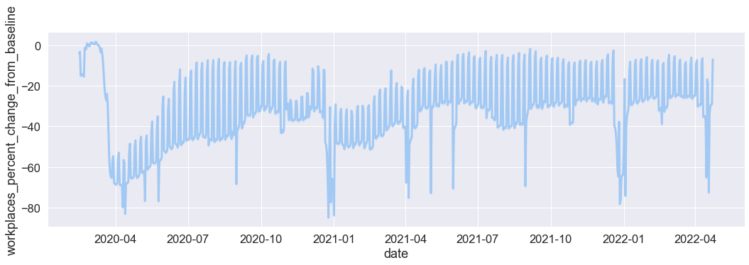
Visualising a single time series variable
A time series is a sequence of data points arranged in time order. We import the seaborn library and use the relplot function to plot the relationship between time and mobility change.
# Import the Seaborn library for data visualisation
import seaborn as sns

%matplotlib inline

sns.set_theme(context="notebook", style="darkgrid", palette="pastel", font_scale=1.5)

sns.relplot(
    x="date",
    y="workplaces_percent_change_from_baseline",
    height=5,
    aspect=3,
    kind="line",
    lw=3,
    data=mobility_trends_UK,
)
<seaborn.axisgrid.FacetGrid at 0x7fef00961e50>
Data wrangling
Transforming from wide to long data format
In the original data, each mobility category is a separate column, which is known as wide data format. Wide data format is easy to read but restricts us to plotting only one mobility category at a time (unless we employ a for loop). We can plot all mobility categories simultaneously in seaborn after we reshape our data from wide format to long format. Long data format will have one column for all six mobility categories and one column for the values of those categories.
Below is a schematic of wide format (left) and long format (right) from the pandas documentation:

We use the pandas melt function to reshape our mobility categories from wide to long format. The function transforms a DataFrame into a format where one or more columns are identifier variables (id_vars), while other columns (value_vars) are turned into a long format, returning columns, ‘variable’ and ‘value’. In our example, id_vars arecountry_region and date, and value_vars are the six mobility categories. The melt function takes the following parameters:
DataFrame— your pandas DataFrameid_vars— a list of identifier variablesvalue_vars— a list of variables to turn into long format
At the end we use the Pandas method dropna() to remove missing values in the DataFrame.
# Transform from wide to long format using the function melt
mobility_trends_UK_long = pd.melt(
    mobility_trends_UK,
    id_vars=mobility_trends_UK.columns[[1, 2, 8]],
    value_vars=mobility_trends_UK.columns[9:15],
).dropna()

mobility_trends_UK_long
| country_region | sub_region_1 | date | variable | value | |
|---|---|---|---|---|---|
| 799 | United Kingdom | Aberdeen City | 2020-02-15 | retail_and_recreation_percent_change_from_base... | -3.0 |
| 800 | United Kingdom | Aberdeen City | 2020-02-16 | retail_and_recreation_percent_change_from_base... | 6.0 |
| 801 | United Kingdom | Aberdeen City | 2020-02-17 | retail_and_recreation_percent_change_from_base... | 11.0 |
| 802 | United Kingdom | Aberdeen City | 2020-02-18 | retail_and_recreation_percent_change_from_base... | 5.0 |
| 803 | United Kingdom | Aberdeen City | 2020-02-19 | retail_and_recreation_percent_change_from_base... | 2.0 |
| ... | ... | ... | ... | ... | ... |
| 1998871 | United Kingdom | York | 2022-04-19 | residential_percent_change_from_baseline | 7.0 |
| 1998872 | United Kingdom | York | 2022-04-20 | residential_percent_change_from_baseline | 7.0 |
| 1998873 | United Kingdom | York | 2022-04-21 | residential_percent_change_from_baseline | 6.0 |
| 1998874 | United Kingdom | York | 2022-04-22 | residential_percent_change_from_baseline | 6.0 |
| 1998875 | United Kingdom | York | 2022-04-23 | residential_percent_change_from_baseline | 0.0 |
1873346 rows × 5 columns
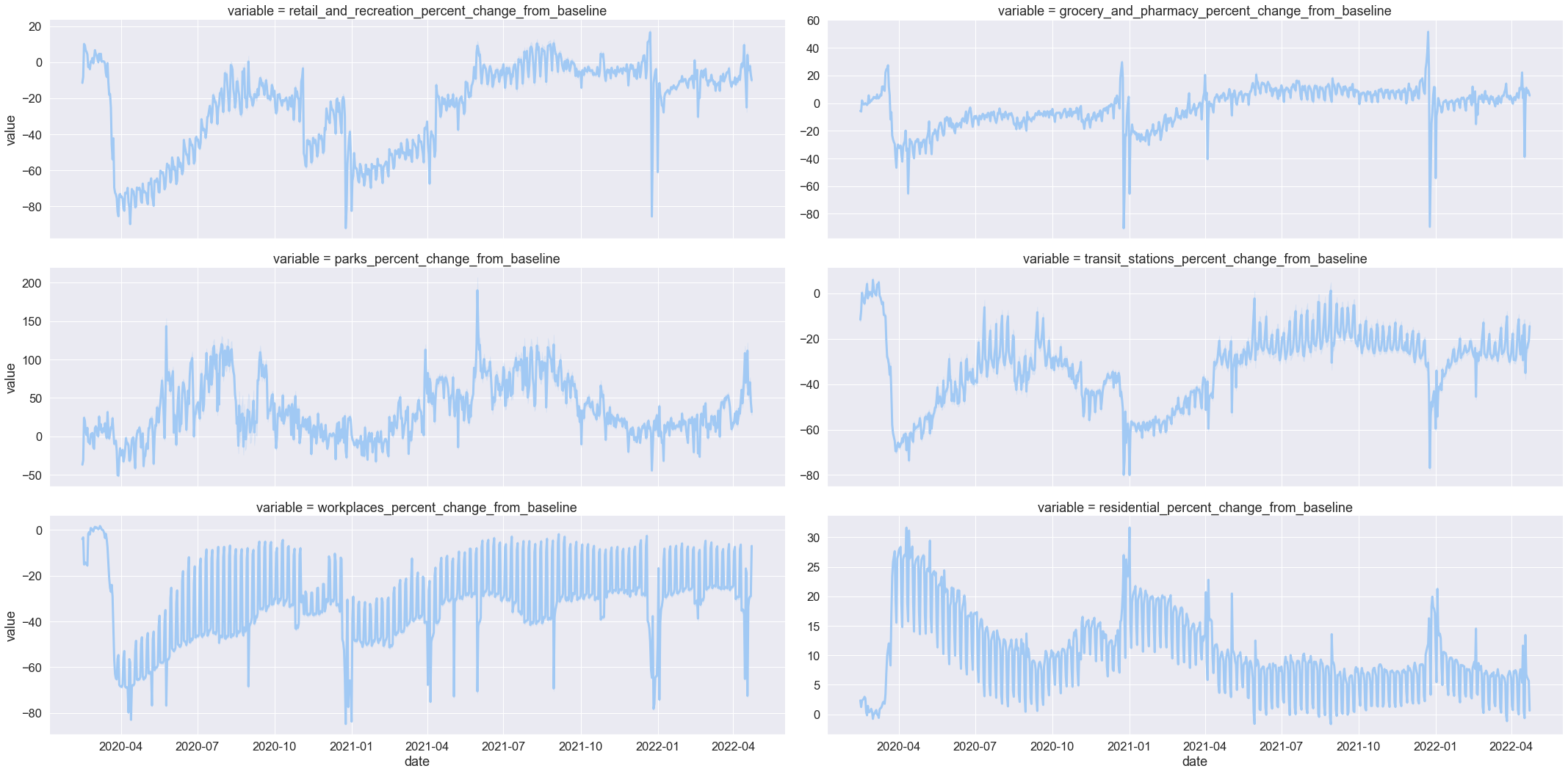
Visualising mobility trends
# Plot the UK time series data for all six mobility categories
sns.relplot(
    x="date",
    y="value",
    col="variable",
    col_wrap=2,
    height=5,
    aspect=3,
    kind="line",
    lw=3,
    facet_kws={"sharey": False},
    data=mobility_trends_UK_long,
)
<seaborn.axisgrid.FacetGrid at 0x7feee9663b80>
Mobility changes across lockdowns
For each lockdown, we consider the first three weeks for comparability.
2020-03-24 — 2020-04-13
2020-11-05 — 2020-11-25
2021-01-06 — 2021-01-26
# Subset data about the three lockdowns
lockdown1 = mobility_trends_UK_long[
    (mobility_trends_UK_long["date"] >= "2020-03-24")
    & (mobility_trends_UK_long["date"] <= "2020-04-13")
]
lockdown2 = mobility_trends_UK_long[
    (mobility_trends_UK_long["date"] >= "2020-11-05")
    & (mobility_trends_UK_long["date"] <= "2020-11-25")
]
lockdown3 = mobility_trends_UK_long[
    (mobility_trends_UK_long["date"] >= "2021-01-06")
    & (mobility_trends_UK_long["date"] <= "2021-01-26")
]

# Link the three DataFrames into one DataFrame
# using the Pandas `concat()` function
lockdowns = pd.concat(
    [lockdown1, lockdown2, lockdown3], keys=["lockdown1", "lockdown2", "lockdown3"]
).reset_index()

lockdowns.head()
| level_0 | level_1 | country_region | sub_region_1 | date | variable | value | |
|---|---|---|---|---|---|---|---|
| 0 | lockdown1 | 837 | United Kingdom | Aberdeen City | 2020-03-24 | retail_and_recreation_percent_change_from_base... | -75.0 |
| 1 | lockdown1 | 838 | United Kingdom | Aberdeen City | 2020-03-25 | retail_and_recreation_percent_change_from_base... | -78.0 |
| 2 | lockdown1 | 839 | United Kingdom | Aberdeen City | 2020-03-26 | retail_and_recreation_percent_change_from_base... | -80.0 |
| 3 | lockdown1 | 840 | United Kingdom | Aberdeen City | 2020-03-27 | retail_and_recreation_percent_change_from_base... | -80.0 |
| 4 | lockdown1 | 841 | United Kingdom | Aberdeen City | 2020-03-28 | retail_and_recreation_percent_change_from_base... | -87.0 |
Split-Apply-Combine
Using the Pandas method groupby(), we split the data into groups (lockdown by mobility category), apply the function mean(), and combine the results.
# Explore descriptive statistics for one of the lockdown DataFrames
lockdowns.groupby(["level_0", "variable"], sort=False)["value"].mean()
level_0    variable
lockdown1  retail_and_recreation_percent_change_from_baseline   -76.643915
           grocery_and_pharmacy_percent_change_from_baseline    -33.936180
           parks_percent_change_from_baseline                   -21.391601
           transit_stations_percent_change_from_baseline        -65.397655
           workplaces_percent_change_from_baseline              -64.930514
           residential_percent_change_from_baseline              25.771162
lockdown2  retail_and_recreation_percent_change_from_baseline   -47.537369
           grocery_and_pharmacy_percent_change_from_baseline    -11.587230
           parks_percent_change_from_baseline                     8.789530
           transit_stations_percent_change_from_baseline        -46.186192
           workplaces_percent_change_from_baseline              -33.901246
           residential_percent_change_from_baseline              14.285984
lockdown3  retail_and_recreation_percent_change_from_baseline   -61.713526
           grocery_and_pharmacy_percent_change_from_baseline    -23.850479
           parks_percent_change_from_baseline                    -9.215003
           transit_stations_percent_change_from_baseline        -58.740466
           workplaces_percent_change_from_baseline              -44.636270
           residential_percent_change_from_baseline              18.332545
Name: value, dtype: float64
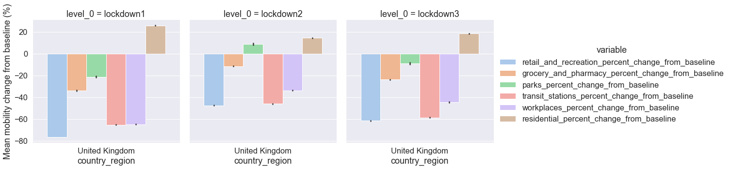
Visual comparison of the three UK lockdowns
# Plot the three lockdowns as a catplot multi-plot
grid = sns.catplot(
    x="country_region",
    y="value",
    hue="variable",
    col="level_0",
    ci=99,
    kind="bar",
    data=lockdowns,
)

grid.set_ylabels("Mean mobility change from baseline (%)")
<seaborn.axisgrid.FacetGrid at 0x7feee9698ee0>
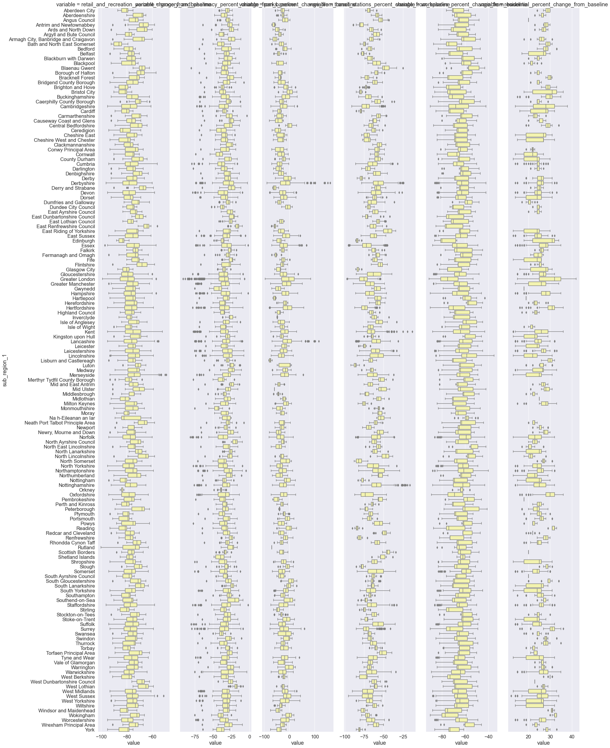
Zooming in: Regional mobility trends
For decision-making and to inform public health interventions, we need to provide results at a higher resolution, for example at the regional level. Below we visualise the six mobility categories across UK regions (counties, districts) during the first lockdown.
# Plot mobility changes across UK regions during the first lockdown
sns.catplot(
    x="value",
    y="sub_region_1",
    col="variable",
    kind="box",
    sharex=False,
    height=35,
    aspect=0.13,
    color="y",
    data=lockdown1,
)
<seaborn.axisgrid.FacetGrid at 0x7fef01749160>
# Plot mobility changes across UK regions during the second lockdown
sns.catplot(
    x="value",
    y="sub_region_1",
    col="variable",
    kind="box",
    sharex=False,
    height=35,
    aspect=0.13,
    color="y",
    data=lockdown2,
)
<seaborn.axisgrid.FacetGrid at 0x7fefced50f70>

# Plot mobility changes across UK regions during the third lockdown
sns.catplot(
    x="value",
    y="sub_region_1",
    col="variable",
    kind="box",
    sharex=False,
    height=35,
    aspect=0.13,
    color="y",
    data=lockdown3,
)
<seaborn.axisgrid.FacetGrid at 0x7fef02056e80>

Re-cap
Using a Colab computational notebook and Python open source tools, we analysed large real-world COVID-19 mobility data through exploratory data analysis and visualisation to address a research question of public health policy relevance.
Accessible hands-on data analysis
We integrated interactive tools and practical hands-on coding that lower barriers to entry for students with little to no programming skills.
Open reproducible research workflow
We combine research question, Python code, explanatory text (comments), exploratory outputs and visualisations in a single document — anyone can check, reproduce, re-use (when we license open source), and improve our analysis.