Python for Data Analysis on the Cloud
Get Started with Jupyter & Colab notebooks
In this course, we will use the Jupyter notebook on the cloud.
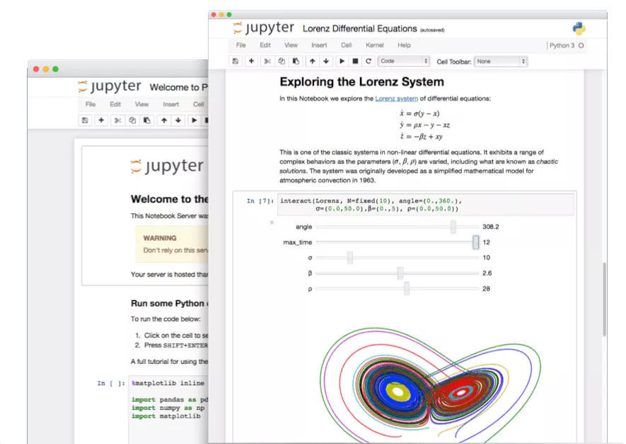
The Jupyter notebook is an open-source web application that allows you to create and share documents that contain live code, equations, visualisations, and narrative text.
There are many free services that allow you to run Jupyter notebooks on the cloud. We will use Colab and Binder.
Colab is a free environment that runs Jupyter notebooks on the Google Cloud and requires no install or setup. You can view notebooks shared publicly without a Google sign-in. In order to execute and change code interactively, a Google account sign-in is required. You can find more information on how to create a Google account here. You can learn more about the Colab and how to open a new notebook here.
MyBinder is a free, community-led infrastructure that opens Jupyter notebooks in an interactive and reproducible environment and requires no install or setup. Binder requires no account registration or log-in to execute and change code interactively.

Learning resources
The Jupyter Notebook. Jupyter Team.
Jupyter Notebook Tutorial. DataCamp.
Get started with Google Colaboratory. Jake VanderPlas, Coding TensorFlow.
A hands-on introduction to Python for beginning programmers. Jessica McKellar, PyCon 2014.
Charles Severance. Python for Everybody: Exploring Data In Python 3.
David Amos et al. Python Basics: A Practical Introduction to Python. The authors make available sample chapters.
Getting Started With the Open Science Framework (OSF). Center for Open Science.
Structure of Colab notebook
The Colab notebook has a simple structure that consists of three parts:
Menubar
Toolbar
Cells
For an example of those features, see an example Colab notebook Overview of Colaboratory Features below.

Manage Jupyter Notebook Files
To open a new notebook:
File -> New notebook
To rename a notebook:
File -> Rename notebook
To access revision history:
File -> Revision history
To check whether the cells in your notebook are executable in linear order:
Runtime -> Restart and run all
To share your Colab notebook and collaborate, you can create a shareable link by clicking the Share button at the top right of your Colab notebook and specify the type of access (e.g., Anyone with the link can view the notebook). You can then copy and share the link with your collaborators.
Cells
The notebook has two types of cells: code and text. You can add new cells by using the + Code and + Text buttons that are in the toolbar above the notebook and also appear when you hover between a pair of cells.
Python Coding for Data Analysis
Below is a code cell, in which we type in the arithmetic expression 21 + 21.
The code is prefixed by a comment. Commenting your code is a good practice and part of your reproducible workflow. Comments in Python’s code cells start with a hashtag symbol # followed by a single space and some text. The text that follows the hashtag symbol on the same line is marked as a comment and is not therefore evaluated by the Python interpreter. Only the code (in this instance, “21 + 21”) is evaluated and the output (in this instance, “42”) will be displayed below the code cell.
To execute the cell, press Shift + Enter or click the Play icon on the left.
# Perform a basic arithmetic operation of addition
21 + 21
42
Python reads the code entered in the cell, evaluates it, and prints the result (42).
Create a toy data set and perform basic data analysis
Let’s create a list of the whole numbers (or integers) 4, 2, 8, 6.
Lists are one of the built-in data types in Python. Elements in a list are separated by comma , and are enclosed in square brackets []:
[4, 2, 8, 6] # create a list
[4, 2, 8, 6]
The comment # create a list is an example of an inline comment. Inline comments refers to a code statement on the same line. Inline comments are separated by at least two spaces from the code statement. Similar to block comments, inline comments start with a hashtag symbol # followed by a single space and some text.
Let’s assign the list of numbers to a variable called even_numbers using the =, which is called the assignment operator.
even_numbers = [4, 2, 8, 6]
You can now apply built-in functions from the Python Standard Library to the variable even_numbers. A function is a block of code that:
takes input parameters
performs a specific task
returns an output.
Python has various built-in functions, including min(), max(), sorted(). Take the function min(). Using our example of even numbers above, the function min() will take as an input parameter the four numbers to compare, perform the comparison, and return the number with the lowest value.
We call a function by writing the function name followed by parenthesis. The function min() takes only one input parameter, the input data in the form of a list or another Python data type we will discuss later in the course. When we call the function, we pass our list even_numbers as an argument inside the parentheses.
An argument is different from a parameter, although the two terms are often used interchangeably. A parameter is the generic variable listed inside the parentheses of a function, whereas an argument is the actual value or data you pass to the function when you call it.
# Find the number with the lowest value
min(even_numbers)
2
We can apply any other built-in Python function. For example, the max() function returns, intuitively, the number with the highest value.
# Find the number with the highest value
max(even_numbers)
8
The function sorted() returns a sorted list of numbers in increasing order. We assign the resulting sorted list to a variable named sorted_even_numbers:
# Sort numbers in increasing order
sorted_even_numbers = sorted(even_numbers)
sorted_even_numbers
[2, 4, 6, 8]
Functions often have multiple parameters. For example, in addition to your input data, the sorted() function takes two optional parameters. One of these parameters is reverse. If you type in reverse = True, the list will be sorted in descending order:
sorted(even_numbers, reverse=True)
[8, 6, 4, 2]
Our list of even numbers is now sorted in descending order.
Descriptive statistics with NumPy
Functions for scientific computing, data analysis, machine learning, and statistical modeling are not in the Python Standard Library but are part of Python libraries or packages. For example, the Python library NumPy for scientific computing includes functions for computing the mean (average of the numbers) and standard deviation (variation or dispersion of the numbers from the mean).
To use NumPy, we first import the library and, by convention, give it the alias np.
# Import the NumPy library
import numpy as np
Now that we imported the module NumPy as np, you can view help on the module by typing the module alias followed by a question mark ?
np?
We now use np. to append each function we will use from NumPy, for example the functions mean() and std.
# Compute the mean of our list of numbers
np.mean(even_numbers)
5.0
# Compute the standard deviation of our list of numbers
np.std(even_numbers)
2.23606797749979
Getting help
In Jupyter and Colab, you can access help information by using the help() function or a question mark ?. For example, to access help information about a function in the Python Standard Library, such as min(), you type in
help(min)

# Alternatively, you can symply type
min?
Help on built-in function min in module builtins:

min(...)
    min(iterable, *[, default=obj, key=func]) -> value
    min(arg1, arg2, *args, *[, key=func]) -> value

    With a single iterable argument, return its smallest item. The
    default keyword-only argument specifies an object to return if
    the provided iterable is empty.
    With two or more arguments, return the smallest argument.
Note
In Jupyter, you access help by pressing Shift + Tab when you are typing in a cell in edit mode. See this tutorial for the difference between edit mode and command mode.
# Get help about the NumPy function mean()
help(np.mean)
Help on function mean in module numpy:

mean(a, axis=None, dtype=None, out=None, keepdims=<no value>)
    Compute the arithmetic mean along the specified axis.

    Returns the average of the array elements.  The average is taken over
    the flattened array by default, otherwise over the specified axis.
    `float64` intermediate and return values are used for integer inputs.

    Parameters
    ----------
    a : array_like
        Array containing numbers whose mean is desired. If `a` is not an
        array, a conversion is attempted.
    axis : None or int or tuple of ints, optional
        Axis or axes along which the means are computed. The default is to
        compute the mean of the flattened array.

        .. versionadded:: 1.7.0

        If this is a tuple of ints, a mean is performed over multiple axes,
        instead of a single axis or all the axes as before.
    dtype : data-type, optional
        Type to use in computing the mean.  For integer inputs, the default
        is `float64`; for floating point inputs, it is the same as the
        input dtype.
    out : ndarray, optional
        Alternate output array in which to place the result.  The default
        is ``None``; if provided, it must have the same shape as the
        expected output, but the type will be cast if necessary.
        See `ufuncs-output-type` for more details.

    keepdims : bool, optional
        If this is set to True, the axes which are reduced are left
        in the result as dimensions with size one. With this option,
        the result will broadcast correctly against the input array.

        If the default value is passed, then `keepdims` will not be
        passed through to the `mean` method of sub-classes of
        `ndarray`, however any non-default value will be.  If the
        sub-class' method does not implement `keepdims` any
        exceptions will be raised.

    Returns
    -------
    m : ndarray, see dtype parameter above
        If `out=None`, returns a new array containing the mean values,
        otherwise a reference to the output array is returned.

    See Also
    --------
    average : Weighted average
    std, var, nanmean, nanstd, nanvar

    Notes
    -----
    The arithmetic mean is the sum of the elements along the axis divided
    by the number of elements.

    Note that for floating-point input, the mean is computed using the
    same precision the input has.  Depending on the input data, this can
    cause the results to be inaccurate, especially for `float32` (see
    example below).  Specifying a higher-precision accumulator using the
    `dtype` keyword can alleviate this issue.

    By default, `float16` results are computed using `float32` intermediates
    for extra precision.

    Examples
    --------
    >>> a = np.array([[1, 2], [3, 4]])
    >>> np.mean(a)
    2.5
    >>> np.mean(a, axis=0)
    array([2., 3.])
    >>> np.mean(a, axis=1)
    array([1.5, 3.5])

    In single precision, `mean` can be inaccurate:

    >>> a = np.zeros((2, 512*512), dtype=np.float32)
    >>> a[0, :] = 1.0
    >>> a[1, :] = 0.1
    >>> np.mean(a)
    0.54999924

    Computing the mean in float64 is more accurate:

    >>> np.mean(a, dtype=np.float64)
    0.55000000074505806 # may vary
Readability of your Python code
To write readable, consistent, and clean code, it is important to consult the PEP (Python Enhancement Proposal) 8 style guide for Python code. The guide describes the rules for writing a readable Python code. Below are outlined key rules to keep in mind when you write your Python code (for details and examples, check out the PEP 8 style guide).
Naming conventions
Variable names (e.g.,
even_numbers) should be lowercase, with words separated by underscores as necessary to improve readability.Names to avoid (as, in some fonts, they are indistinguishable from the numerals one and zero): the characters ‘l’ (lowercase letter el), ‘O’ (uppercase letter oh), or ‘I’ (uppercase letter eye) as single character variable names.
Comments
PEP 8 distinguishes block comments, inline comments, and documentation strings (or docstrings for short):
Block comments in Python’s code cells apply to the lines of code that follows them, and follow the same indentation as the code. Block comments are typically formed of complete sentences, each sentence starting with a capitalized word and ending in a period. Each line of a block comment starts with a hashtag symbol
#followed by a single space and some text.Line comments appears on the same line as a statement and is separated by at least two spaces from the statement. Each line comment starts with a hashtag symbol
#followed by a single space and some text.Dockstrings are used to document Python modules, functions, classes, or methods. Docstrings are surrounded by
"""triple double quotes""". You likely read docstrings more often (for example, when accessing help information about a function) than write them. See PEP 8 for details on docstrings.
Maximum line length
Limit all lines to a maximum of 79 characters. To split a long command over multiple lines, one can break down code into readable statements using parenthesis. Another approach is to use the backslash symbol
\.Long blocks of text (comments) should be limited to 72 characters.
When applicable and agreed upon, it would be okay to increase the line length limit up to 99 characters, provided that comments are still limited to 72 characters.
Indentation
Indentation in Python is the spaces at the beginning of a code line. Indentation is important not only because of code readability but particularly because in Python statements arranged at the same indentation level are considered to form part of a single code block. So, incorrect indentation in Python would likely produce an IndentationError or an errorless output.
Use 4 spaces per indentation level.
Tabs or Spaces?
Spaces are the preferred indentation method.
Python disallows mixing tabs and spaces for indentation.
Whitespace in Expressions and Statements
Always surround these binary operators with a single space on either side: assignment (=), augmented assignment (+=, -= etc.), comparisons (==, <, >, !=, <>, <=, >=, in, not in, is, is not), Booleans (and, or, not). (e.g.,
sorted_even_numbers = sorted(even_numbers))Don’t use spaces around the
=sign when used to indicate a keyword argument (e.g.,reverse=True)
As mentioned in PEP 8, section A Foolish Consistency is the Hobgoblin of Little Minds, style guide recommendations may not be applicable in some circumstances. In such circumstances, you could look for examples from the Python community and use your best judgment.
Running command-line commands in Jupyter/Colab notebook
In addition to running Python code, we will also execute command-line commands in our Jupyter notebooks. Command-line commands are very useful for obtaining information (for example, you can check the version of your Jupyter notebook, Python, or packages), managing computer files, and installing Python packages.
To execute command-line commands, you would typically need to use a command-line interface (CLI) such as the Terminal (macOS) or Command Prompt (Windows), which can be challenging. Fortunately, Jupyter notebook allows you to run command-line commands in the notebook code cells by prepending an exclamation mark (!) to the beginning of the command. Any command appearing after the mark in the line will not be executed from the Python environment but from your operating system’s command-line interface (CLI). You can think of the exclamation mark (!) as introducing command-line interface (You can learn more about the command-line interfaces from this tutorial by The Carpentries).
As an example, you can determine the version of the Jupyter notebook you use by typing the line below, in which the question mark (!) is followed by the command jupyter-notebook and the flag --version. Command-line flags are used to specify options and modify command’s execution. As an output, the command prints the version of your active Jupyter notebook.
!jupyter-notebook --version
6.1.4
Installing packages with pip
Command-line tools are particularly useful for installing packages that are not part of the Python standard library. To install packages, we will use the Python’s packaging manager pip. A list of all Python packages available for instalation via pip can be found at https://pypi.org.
Because pip is a command-line tool, we will prepend an exclamation mark (!) to the package installation command every time we use pip. The pip install command supports flags, for example we will specify the flag -q (short for --quiet) that hides output/warnings which may cause confusion initially. For example, to install the Python package for statistical modeling, statsmodels, we would type:
!pip install -q statsmodels
The command above installs the most recent version of a package, which you can determine (along other useful information about the package) by typing:
!pip show statsmodels
Name: statsmodels
Version: 0.12.2
Summary: Statistical computations and models for Python
Home-page: https://www.statsmodels.org/
Author:
Author-email:
License: BSD License
Location: /Users/valentindanchev/opt/anaconda3/lib/python3.8/site-packages
Requires: numpy, pandas, patsy, scipy
Required-by: dowhy
If you are interested in installing a previous version of statsmodels (for example, for the purpose of reproducing a research project which uses a previous version), you can find the available previous versions at https://pypi.org and install a version of choice by typing the version number, for example:
!pip install -q statsmodels==0.12.2
Jupyter magic commands
Jupyter magic commands are special commands that add to the Python syntax and provide capabilities that help researchers solve various research problems related to data analysis and workflow. Magic commands are prefixed in the Jupyter notebook by a single % character when they operate on one line of code (known as line magics) or by double %% characters when they operate on multiple lines of code (known as cell magics).
You can list all available magic commands by using the line magic %lsmagic as shown below.
%lsmagic
Available line magics:
%alias  %alias_magic  %autoawait  %autocall  %automagic  %autosave  %bookmark  %cat  %cd  %clear  %colors  %conda  %config  %connect_info  %cp  %debug  %dhist  %dirs  %doctest_mode  %ed  %edit  %env  %gui  %hist  %history  %killbgscripts  %ldir  %less  %lf  %lk  %ll  %load  %load_ext  %loadpy  %logoff  %logon  %logstart  %logstate  %logstop  %ls  %lsmagic  %lx  %macro  %magic  %man  %matplotlib  %mkdir  %more  %mv  %notebook  %page  %pastebin  %pdb  %pdef  %pdoc  %pfile  %pinfo  %pinfo2  %pip  %popd  %pprint  %precision  %prun  %psearch  %psource  %pushd  %pwd  %pycat  %pylab  %qtconsole  %quickref  %recall  %rehashx  %reload_ext  %rep  %rerun  %reset  %reset_selective  %rm  %rmdir  %run  %save  %sc  %set_env  %store  %sx  %system  %tb  %time  %timeit  %unalias  %unload_ext  %who  %who_ls  %whos  %xdel  %xmode

Available cell magics:
%%!  %%HTML  %%SVG  %%bash  %%capture  %%debug  %%file  %%html  %%javascript  %%js  %%latex  %%markdown  %%perl  %%prun  %%pypy  %%python  %%python2  %%python3  %%ruby  %%script  %%sh  %%svg  %%sx  %%system  %%time  %%timeit  %%writefile

Automagic is ON, % prefix IS NOT needed for line magics.
Some of the popular magic commands we will use include:
Printing out the execution time of a Python command
%time np.mean(even_numbers)
CPU times: user 77 µs, sys: 41 µs, total: 118 µs
Wall time: 121 µs
5.0
Listing all variables already defined in the current notebook
%who
even_numbers np sorted_even_numbers
Displaying matlpotlib/Seaborn graphs in the notebook (applies to older versions of Jupyter notebook, obsolete in newer versions)
%matplotlib inline
You can read more about the Jupyter magic commands here and here.

Loading real-world data with pandas
So far, we have used a toy data example. We will use the pandas library to load a real-world data set. We will learn about pandas next session, here will just use key data loading functionality. Let’s first import the pandas library and, by convention, give it the alias pd.
# Import the pandas library
import pandas as pd
Data on Covid-19 by Our World in Data
We will load and explore the Data on COVID-19 by Our World in Data (OWID). Details about the data are available on this GitHub repository:
It is updated daily and includes data on confirmed cases, deaths, hospitalizations, testing, and vaccinations as well as other variables of potential interest.
The data on COVID-19 by Our World in Data is provided as a comma-separated values (CSV) file. We load the CSV file into Python using the read_csv() function from pandas. There is no need to download the file on your local computer or the cloud. We just specify the URL and use the code below to load the most recent online version of the data. We also assign the loaded data set to a variable called owid_covid.
owid_covid = pd.read_csv("https://covid.ourworldindata.org/data/owid-covid-data.csv")
We can now perform various operations on the data object by using the so called methods. Examples of pandas methods are head() and tail(); head() displays by default the top five rows of the data and tail() displays by default the last five rows. You can display a custom number of row by passing that number in in the brackets.
Let’s display the top five rows using the method head():
# View the top five rows of the data set
owid_covid.head()
| iso_code | continent | location | date | total_cases | new_cases | new_cases_smoothed | total_deaths | new_deaths | new_deaths_smoothed | ... | female_smokers | male_smokers | handwashing_facilities | hospital_beds_per_thousand | life_expectancy | human_development_index | excess_mortality_cumulative_absolute | excess_mortality_cumulative | excess_mortality | excess_mortality_cumulative_per_million | |
|---|---|---|---|---|---|---|---|---|---|---|---|---|---|---|---|---|---|---|---|---|---|
| 0 | AFG | Asia | Afghanistan | 2020-02-24 | 5.0 | 5.0 | NaN | NaN | NaN | NaN | ... | NaN | NaN | 37.746 | 0.5 | 64.83 | 0.511 | NaN | NaN | NaN | NaN |
| 1 | AFG | Asia | Afghanistan | 2020-02-25 | 5.0 | 0.0 | NaN | NaN | NaN | NaN | ... | NaN | NaN | 37.746 | 0.5 | 64.83 | 0.511 | NaN | NaN | NaN | NaN |
| 2 | AFG | Asia | Afghanistan | 2020-02-26 | 5.0 | 0.0 | NaN | NaN | NaN | NaN | ... | NaN | NaN | 37.746 | 0.5 | 64.83 | 0.511 | NaN | NaN | NaN | NaN |
| 3 | AFG | Asia | Afghanistan | 2020-02-27 | 5.0 | 0.0 | NaN | NaN | NaN | NaN | ... | NaN | NaN | 37.746 | 0.5 | 64.83 | 0.511 | NaN | NaN | NaN | NaN |
| 4 | AFG | Asia | Afghanistan | 2020-02-28 | 5.0 | 0.0 | NaN | NaN | NaN | NaN | ... | NaN | NaN | 37.746 | 0.5 | 64.83 | 0.511 | NaN | NaN | NaN | NaN |
5 rows × 67 columns
# View the last five rows of the data set
owid_covid.tail()
| iso_code | continent | location | date | total_cases | new_cases | new_cases_smoothed | total_deaths | new_deaths | new_deaths_smoothed | ... | female_smokers | male_smokers | handwashing_facilities | hospital_beds_per_thousand | life_expectancy | human_development_index | excess_mortality_cumulative_absolute | excess_mortality_cumulative | excess_mortality | excess_mortality_cumulative_per_million | |
|---|---|---|---|---|---|---|---|---|---|---|---|---|---|---|---|---|---|---|---|---|---|
| 189721 | ZWE | Africa | Zimbabwe | 2022-05-23 | 250702.0 | 60.0 | 181.571 | 5495.0 | 1.0 | 1.571 | ... | 1.6 | 30.7 | 36.791 | 1.7 | 61.49 | 0.571 | NaN | NaN | NaN | NaN |
| 189722 | ZWE | Africa | Zimbabwe | 2022-05-24 | 250929.0 | 227.0 | 168.714 | 5496.0 | 1.0 | 1.714 | ... | 1.6 | 30.7 | 36.791 | 1.7 | 61.49 | 0.571 | NaN | NaN | NaN | NaN |
| 189723 | ZWE | Africa | Zimbabwe | 2022-05-25 | 251228.0 | 299.0 | 174.429 | 5496.0 | 0.0 | 1.429 | ... | 1.6 | 30.7 | 36.791 | 1.7 | 61.49 | 0.571 | NaN | NaN | NaN | NaN |
| 189724 | ZWE | Africa | Zimbabwe | 2022-05-26 | 251646.0 | 418.0 | 205.714 | 5498.0 | 2.0 | 1.571 | ... | 1.6 | 30.7 | 36.791 | 1.7 | 61.49 | 0.571 | NaN | NaN | NaN | NaN |
| 189725 | ZWE | Africa | Zimbabwe | 2022-05-27 | 251959.0 | 313.0 | 212.857 | 5500.0 | 2.0 | 1.571 | ... | 1.6 | 30.7 | 36.791 | 1.7 | 61.49 | 0.571 | NaN | NaN | NaN | NaN |
5 rows × 67 columns
Describe the Covid-19 data
In addition to pandas methods, we can use attributes to access information about the metadata. For example, the attribute shape gives the dimensions of a DataFrame.
# Number of rows and columns in the data set
owid_covid_shape = owid_covid.shape
owid_covid_shape
(189726, 67)
The returned object is called tuples. Like lists, tuples contain a collection of data elements. But unlike lists, which are mutable, tuples are immutable, meaning that the element values cannot change. Also, compared to lists in which elements are inside square brackets [], elements in tuples are inside parentheses ().
To access a particular value in tuple, we use the square brackets. For example, to access the first element (i.e., number of rows) of the tuple owid_covid_shape, we type in
owid_covid_shape[0]
189726
To access the second element (i.e., number of columns) of the tuple, we type in
owid_covid.shape[1]
67
Note that indexing in Python starts from 0, so first element is index 0, second is index 1, and so on.
As of 11 May 2021, the data set contains 87,310 rows and 59 columns. But this is a live data set in which the number of rows are updated daily. To display these updates, we could use the print() function. The line of code below contains background text in quotes '' and the up-to-date number of rows owid_covid.shape[0] and number of columns owid_covid.shape[1] that will be inserted in the sentence each time the cell is executed.
print(
    "In the most current data on COVID-19 by Our World in Data, the number of rows is",
    owid_covid.shape[0],
    "and the number of columns is",
    owid_covid.shape[1],
)
In the most current data on COVID-19 by Our World in Data, the number of rows is 189726 and the number of columns is 67
In addition to the dimensions of the data set, we can access other metadata using attributes. For example, we can access the column labels of the data set using the attribute columns:
owid_covid.columns
Index(['iso_code', 'continent', 'location', 'date', 'total_cases', 'new_cases',
       'new_cases_smoothed', 'total_deaths', 'new_deaths',
       'new_deaths_smoothed', 'total_cases_per_million',
       'new_cases_per_million', 'new_cases_smoothed_per_million',
       'total_deaths_per_million', 'new_deaths_per_million',
       'new_deaths_smoothed_per_million', 'reproduction_rate', 'icu_patients',
       'icu_patients_per_million', 'hosp_patients',
       'hosp_patients_per_million', 'weekly_icu_admissions',
       'weekly_icu_admissions_per_million', 'weekly_hosp_admissions',
       'weekly_hosp_admissions_per_million', 'total_tests', 'new_tests',
       'total_tests_per_thousand', 'new_tests_per_thousand',
       'new_tests_smoothed', 'new_tests_smoothed_per_thousand',
       'positive_rate', 'tests_per_case', 'tests_units', 'total_vaccinations',
       'people_vaccinated', 'people_fully_vaccinated', 'total_boosters',
       'new_vaccinations', 'new_vaccinations_smoothed',
       'total_vaccinations_per_hundred', 'people_vaccinated_per_hundred',
       'people_fully_vaccinated_per_hundred', 'total_boosters_per_hundred',
       'new_vaccinations_smoothed_per_million',
       'new_people_vaccinated_smoothed',
       'new_people_vaccinated_smoothed_per_hundred', 'stringency_index',
       'population', 'population_density', 'median_age', 'aged_65_older',
       'aged_70_older', 'gdp_per_capita', 'extreme_poverty',
       'cardiovasc_death_rate', 'diabetes_prevalence', 'female_smokers',
       'male_smokers', 'handwashing_facilities', 'hospital_beds_per_thousand',
       'life_expectancy', 'human_development_index',
       'excess_mortality_cumulative_absolute', 'excess_mortality_cumulative',
       'excess_mortality', 'excess_mortality_cumulative_per_million'],
      dtype='object')
Display a concise summary of the DataFrame using the method info()
owid_covid.info()
<class 'pandas.core.frame.DataFrame'>
RangeIndex: 189726 entries, 0 to 189725
Data columns (total 67 columns):
 #   Column                                      Non-Null Count   Dtype
---  ------                                      --------------   -----
 0   iso_code                                    189726 non-null  object
 1   continent                                   178691 non-null  object
 2   location                                    189726 non-null  object
 3   date                                        189726 non-null  object
 4   total_cases                                 182231 non-null  float64
 5   new_cases                                   182021 non-null  float64
 6   new_cases_smoothed                          180847 non-null  float64
 7   total_deaths                                163807 non-null  float64
 8   new_deaths                                  163798 non-null  float64
 9   new_deaths_smoothed                         162635 non-null  float64
 10  total_cases_per_million                     181390 non-null  float64
 11  new_cases_per_million                       181180 non-null  float64
 12  new_cases_smoothed_per_million              180011 non-null  float64
 13  total_deaths_per_million                    162979 non-null  float64
 14  new_deaths_per_million                      162970 non-null  float64
 15  new_deaths_smoothed_per_million             161812 non-null  float64
 16  reproduction_rate                           140710 non-null  float64
 17  icu_patients                                25287 non-null   float64
 18  icu_patients_per_million                    25287 non-null   float64
 19  hosp_patients                               26547 non-null   float64
 20  hosp_patients_per_million                   26547 non-null   float64
 21  weekly_icu_admissions                       6147 non-null    float64
 22  weekly_icu_admissions_per_million           6147 non-null    float64
 23  weekly_hosp_admissions                      12267 non-null   float64
 24  weekly_hosp_admissions_per_million          12267 non-null   float64
 25  total_tests                                 77125 non-null   float64
 26  new_tests                                   73556 non-null   float64
 27  total_tests_per_thousand                    77125 non-null   float64
 28  new_tests_per_thousand                      73556 non-null   float64
 29  new_tests_smoothed                          99918 non-null   float64
 30  new_tests_smoothed_per_thousand             99918 non-null   float64
 31  positive_rate                               92182 non-null   float64
 32  tests_per_case                              90545 non-null   float64
 33  tests_units                                 102647 non-null  object
 34  total_vaccinations                          51818 non-null   float64
 35  people_vaccinated                           49369 non-null   float64
 36  people_fully_vaccinated                     46824 non-null   float64
 37  total_boosters                              23926 non-null   float64
 38  new_vaccinations                            42442 non-null   float64
 39  new_vaccinations_smoothed                   102364 non-null  float64
 40  total_vaccinations_per_hundred              51818 non-null   float64
 41  people_vaccinated_per_hundred               49369 non-null   float64
 42  people_fully_vaccinated_per_hundred         46824 non-null   float64
 43  total_boosters_per_hundred                  23926 non-null   float64
 44  new_vaccinations_smoothed_per_million       102364 non-null  float64
 45  new_people_vaccinated_smoothed              101351 non-null  float64
 46  new_people_vaccinated_smoothed_per_hundred  101351 non-null  float64
 47  stringency_index                            147714 non-null  float64
 48  population                                  188568 non-null  float64
 49  population_density                          169064 non-null  float64
 50  median_age                                  156690 non-null  float64
 51  aged_65_older                               155029 non-null  float64
 52  aged_70_older                               155868 non-null  float64
 53  gdp_per_capita                              155859 non-null  float64
 54  extreme_poverty                             101750 non-null  float64
 55  cardiovasc_death_rate                       156337 non-null  float64
 56  diabetes_prevalence                         163976 non-null  float64
 57  female_smokers                              118246 non-null  float64
 58  male_smokers                                116625 non-null  float64
 59  handwashing_facilities                      76812 non-null   float64
 60  hospital_beds_per_thousand                  138717 non-null  float64
 61  life_expectancy                             177427 non-null  float64
 62  human_development_index                     152298 non-null  float64
 63  excess_mortality_cumulative_absolute        6525 non-null    float64
 64  excess_mortality_cumulative                 6525 non-null    float64
 65  excess_mortality                            6525 non-null    float64
 66  excess_mortality_cumulative_per_million     6525 non-null    float64
dtypes: float64(62), object(5)
memory usage: 97.0+ MB
Let’s see what is the highest number of fully vaccinated adults in a country to date. We will use the variable people_fully_vaccinated_per_hundred and pandas’ max() method.
owid_covid["people_fully_vaccinated_per_hundred"].max()
122.94
Once we know the highest number of fully vaccinated adults per hundred, we determine the index of the observation (country) associated with that number using the pandas’ method idmax().
index_highest_vaccination = owid_covid["people_fully_vaccinated_per_hundred"].idxmax()
index_highest_vaccination
66501
Finally, we select the particular row (country in this case) by its location in the index using iloc.
owid_covid.iloc[[index_highest_vaccination]]
| iso_code | continent | location | date | total_cases | new_cases | new_cases_smoothed | total_deaths | new_deaths | new_deaths_smoothed | ... | female_smokers | male_smokers | handwashing_facilities | hospital_beds_per_thousand | life_expectancy | human_development_index | excess_mortality_cumulative_absolute | excess_mortality_cumulative | excess_mortality | excess_mortality_cumulative_per_million | |
|---|---|---|---|---|---|---|---|---|---|---|---|---|---|---|---|---|---|---|---|---|---|
| 66501 | GIB | Europe | Gibraltar | 2022-04-21 | 17706.0 | 212.0 | 30.286 | 101.0 | 0.0 | 0.0 | ... | NaN | NaN | NaN | NaN | 79.93 | NaN | NaN | NaN | NaN | NaN |
1 rows × 67 columns
The above example is only for illustration of pandas functionality. We will unpack different approaches for data slicing and selecting with pandas in section Data Design and Data Wrangling.
Hands-on exercise: Let’s practice your Python skills
Open a new
Colabnotebook.Add a new
Codecell and include the following:Import the pandas library and add a comment describing your code
Load the Data on COVID-19 by Our World in Data and assign the data to a variable name. Use an informative variable name that clearly describes what the data is about; you can use underscores to separate words in your variable name, e.g. COVID19_Data_Our_World_in_Data. Add a comment.
For the loaded data set:
Show the first 20 observations/rows
Show the last 5 observations/rows
When ready, share your Colab notebook with the class:
Create a shareable link by clicking the Share button at the top right of your Colab notebook
Specify that Anyone with the link can view the notebook
Share the link with the class.
Before sharing your notebook, rerun your notebook from top to bottom using Restart and run all (under Runtime in the Colab menu bar) to ensure that your data analysis is computationally reproducible.
Markdown Text Cells
Double click a text cell to see the Markdown syntax used to format the text.
Headings
Headings begin with the hash symbol ‘#,’ followed by the space. There are six Headings. To create the largest heading, add one hash symbol, and to create the smallest heading, add six hash symbols.
# Header 1, Title example (Not shown below)
## Header 2, Subtitle example
### Header 3,
#### Header 4
##### etc.
Lists
* Item one (Note the space after *)
* Item two
* Item three
  * Sub-bullet
    * Sub-sub-bullet
Item one
Item two
Item three
Sub-bullet
Sub-sub-bullet
Bold and Italic Text
**This text is bold**
*This text is italic*
~This was mistaken text~
***This is both bold and italic text***
This text is bold
This text is italic
A second line of stricken code
This is both bold and italic text
Hyperlinks
Markdown allows you to create links to content on the web using the following syntax:
[Link title](https://)
For example, a hyperlink to the Project Jupyter would look like that:
[Project Jupyter](https://jupyter.org)
Hands-on exercise: Let’s practice your Markdown skills
Create a new
Colabnotebook file.Add a new
Textcell and include:
A notebook title (e.g. My Reproducible Research Workflow)
A bullet list with:
A bold word for
Author: and then add italised text for your name.A bold word for
Affiliation: and then add italised text for your University and Department.A bold word for
Date: and then add text for today’s date.
Add another Text cell and include:
A list of at least two online datasets about Covid-19 you find interesting.
Add a hyperlink to each database in your list and include the name of the database in the title of the hyperlink.
Add another Text cell and write a short research question you would be interesting in addressing using the Covid-19 datasets.
When you complete your exercise, download your notebook and make it available on an Open Science Framework (OSF) repository. You can download your Colab notebook from File and then Download .ipynb. You can learn how to create an OSF repository and deposit your notebook from the tutorial Getting Started With the Open Science Framework by the Center for Open Science.
This exercise draws on Earth Lab’s lesson Format Text In Jupyter Notebook With Markdown.