Exploratory Data Analysis and Visualisation
The term Exploratory Data Analysis (EDA) was introduced by John Tukey in his book of the same title published in 1977. It is an approach of data analysis in which you employ a number of simple quantitative techniques (for example, descriptive statistics like the mean and the standard deviation) and visualisation to explore features of the data with an ‘open mind’, before any particular statistical assumptions and models are applied to the data.
“‘Exploratory data analysis’ is an attitude, a state of flexibility, a willingness to look for those things that we believe are not there, as well as those we believe to be there.” — John Tukey, 1977
EDA can be seen as a paradigm of data analysis emphasising the ‘flexibility’ of data exploration and visualisation and the ability of a researcher to adapt to the ‘clues’ the data may reveal. Note that EDA is performed before data modelling. EDA is therefore different from any data exploration after the outputs from initial modelling are known, which is typically not regarded as a good research practice, unless openly reported. Such post-modelling exploration would likely motivate additional tests that are arbitrary yet could produce positive and statistically significant results (See Simmons, Nelson, and Simonsohn, 2011).
In this lab, we will explore and visualise various features and patterns in the mobility trends data using the Python libraries pandas for data analysis and SciPy and NumPy for descriptive statistics and simple modelling. We will introduce the library Seaborn for data visualisation. Seaborn is a Python data visualisation library built on top of matplotlib. It provides an interface for drawing attractive and informative statistical graphics.
We formulate simple research questions (RQ) and employ EDA to shed light on features of data that can help us address those research questions. We will perform various visualizations to communicate quantitative features, patterns, and longitudinal trends in our data. We will discuss good research practices related to EDA and visualisation.
Learning resources
Sam Lau, Joey Gonzalez, and Deb Nolan. 10.4. Visualization Principles. In Principles and Techniques of Data Science.
Kieran Healy and James Moody. Data Visualization in Sociology. Annual Review of Sociology.
Misleading Axes and Manipulating Bin Sizes, part of the course Calling Bullshit by Carl T. Bergstrom and Jevin West
Introduction to Data Processing in Python with Pandas, SciPy 2019 Tutorial by Daniel Chen (The visualisation library Seaborn is covered in the video between 2:15 and 2:45)
Addressing simple questions via Python EDA
Importing libraries
We first import Python libraries for exploratory data analysis and visualisation. We also import the libraries Statsmodels and SciPy for statistical and scientific computing, which we will use to fit simple statistical models after our data explorations.
# Import Python libraries for visualisation and data analysis
import matplotlib.pyplot as plt
import numpy as np
import pandas as pd
import seaborn as sns

sns.set_theme()  # Apply the default Seaborn theme
%matplotlib inline

# Suppress warnings to avoid potential confusion
import warnings

# Libraries for statistical and scientific computing
import statsmodels.api as sm
from scipy import stats

warnings.filterwarnings("ignore")
Loading and processing the COVID-19 mobility data
# Load the Covid-19 Google Community Mobility Reports
# By default, Pandas will read the date column as string, so we use parse_dates to
# convert the string into datetimes we will use for time series plots.
mobility_trends_complete = pd.read_csv(
    "https://www.gstatic.com/covid19/mobility/Global_Mobility_Report.csv",
    parse_dates=["date"],
)

# The Community Mobility Reports is updated daily, approaching
# 10 million rows as of April 2022. To make data analysis more
# manageable, we select a subset of the dataset until 30 June 2021
# (15 February 2020 is the first time point in the data set).
mobility_trends = mobility_trends_complete[
    mobility_trends_complete["date"].isin(
        pd.date_range(start="2020-02-15", end="2021-06-30")
    )
]

# Rename (i.e., shorten the labels) the six mobility categories
mobility_trends.rename(
    columns={
        "retail_and_recreation_percent_change_from_baseline": "Retail_Recreation",
        "grocery_and_pharmacy_percent_change_from_baseline": "Grocery_Pharmacy",
        "parks_percent_change_from_baseline": "Parks",
        "transit_stations_percent_change_from_baseline": "Transit_stations",
        "workplaces_percent_change_from_baseline": "Workplaces",
        "residential_percent_change_from_baseline": "Residential",
    },
    inplace=True,
)

mobility_trends
Code reuse: creating your own functions
We will need to pre-process the mobility data in subsequent chapters as well. Instead of typing (or copying and pasting) the lines of code for pre-processing multiple times, which would likely introduce errors, it is a good practice to define your own function that stores your code. You can then call that function when you need to reuse the code. Below we define two functions called subperiod_mobility_trends and rename_mobility_trends which we will use in the next lesson to process the mobility data.
Let’s use the subperiod_mobility_trends as an example. As every function (see the book Python Basics: A Practical Introduction to Python 3), subperiod_mobility_trends has three parts:
function signature
docstring (short for documentation strings)
function body
Let’s describe each of these three parts.
The function signature has the following four components:
the
defkeyword (short for define)the function name,
subperiod_mobility_trendsthe list of parameters,
data,start_date, andend_date(these are placeholders for the actual data and start and end dates we will provide when we call the function)A colon (:) at the end of the line of code.
The docstring is placed immediately after the function definition (the function signature), enclosed in triple-double quotes (“””). The purpose of the dosctrings is to document the code and to state its main purpose.
The function body consists of the code that runs when you call the function. For example, the function body for subperiod_mobility_trends consists of a block of code that selects a subset of the mobility data for a period of time with pre-specified start date and end date.
Let’s define our function for selecting mobility trends for a subperiod and save the function as subperiod_mobility_trends.py so that we can reuse the code in subsequent notebooks.
def subperiod_mobility_trends(data, start_date, end_date):
    """
    Add your mobility data in `data`.

    This function selects a subperiod of the mobility data based on prespecified start data and end date.
    """
    mobility_trends = data[
        data["date"].isin(pd.date_range(start=start_date, end=end_date))
    ]
    return mobility_trends


def rename_mobility_trends(data):
    """
    This function renames the column headings of the six mobility categories.
    """
    mobility_trends_renamed = data.rename(
        columns={
            "retail_and_recreation_percent_change_from_baseline": "Retail_Recreation",
            "grocery_and_pharmacy_percent_change_from_baseline": "Grocery_Pharmacy",
            "parks_percent_change_from_baseline": "Parks",
            "transit_stations_percent_change_from_baseline": "Transit_stations",
            "workplaces_percent_change_from_baseline": "Workplaces",
            "residential_percent_change_from_baseline": "Residential",
        }
    )
    return mobility_trends_renamed
Let’s call our functions. We pass as input to the function subperiod_mobility_trends() the complete Community Mobility Reports data set we already loaded as mobility_trends_complete. We then pass the output as input to the function rename_mobility_trends().
mobility_trends = subperiod_mobility_trends(
    mobility_trends_complete, "2020-02-15", "2021-06-30"
)

mobility_trends = rename_mobility_trends(mobility_trends)

mobility_trends
| country_region_code | country_region | sub_region_1 | sub_region_2 | metro_area | iso_3166_2_code | census_fips_code | place_id | date | Retail_Recreation | Grocery_Pharmacy | Parks | Transit_stations | Workplaces | Residential | |
|---|---|---|---|---|---|---|---|---|---|---|---|---|---|---|---|
| 0 | AE | United Arab Emirates | NaN | NaN | NaN | NaN | NaN | ChIJvRKrsd9IXj4RpwoIwFYv0zM | 2020-02-15 | 0.0 | 4.0 | 5.0 | 0.0 | 2.0 | 1.0 |
| 1 | AE | United Arab Emirates | NaN | NaN | NaN | NaN | NaN | ChIJvRKrsd9IXj4RpwoIwFYv0zM | 2020-02-16 | 1.0 | 4.0 | 4.0 | 1.0 | 2.0 | 1.0 |
| 2 | AE | United Arab Emirates | NaN | NaN | NaN | NaN | NaN | ChIJvRKrsd9IXj4RpwoIwFYv0zM | 2020-02-17 | -1.0 | 1.0 | 5.0 | 1.0 | 2.0 | 1.0 |
| 3 | AE | United Arab Emirates | NaN | NaN | NaN | NaN | NaN | ChIJvRKrsd9IXj4RpwoIwFYv0zM | 2020-02-18 | -2.0 | 1.0 | 5.0 | 0.0 | 2.0 | 1.0 |
| 4 | AE | United Arab Emirates | NaN | NaN | NaN | NaN | NaN | ChIJvRKrsd9IXj4RpwoIwFYv0zM | 2020-02-19 | -2.0 | 0.0 | 4.0 | -1.0 | 2.0 | 1.0 |
| ... | ... | ... | ... | ... | ... | ... | ... | ... | ... | ... | ... | ... | ... | ... | ... |
| 9709045 | ZW | Zimbabwe | Midlands Province | Kwekwe | NaN | NaN | NaN | ChIJRcIZ3-FJNBkRRsj55IcLpfU | 2021-06-24 | NaN | NaN | NaN | NaN | 7.0 | NaN |
| 9709046 | ZW | Zimbabwe | Midlands Province | Kwekwe | NaN | NaN | NaN | ChIJRcIZ3-FJNBkRRsj55IcLpfU | 2021-06-25 | NaN | NaN | NaN | NaN | 13.0 | NaN |
| 9709047 | ZW | Zimbabwe | Midlands Province | Kwekwe | NaN | NaN | NaN | ChIJRcIZ3-FJNBkRRsj55IcLpfU | 2021-06-28 | NaN | NaN | NaN | NaN | -3.0 | NaN |
| 9709048 | ZW | Zimbabwe | Midlands Province | Kwekwe | NaN | NaN | NaN | ChIJRcIZ3-FJNBkRRsj55IcLpfU | 2021-06-29 | NaN | NaN | NaN | NaN | 12.0 | NaN |
| 9709049 | ZW | Zimbabwe | Midlands Province | Kwekwe | NaN | NaN | NaN | ChIJRcIZ3-FJNBkRRsj55IcLpfU | 2021-06-30 | NaN | NaN | NaN | NaN | 5.0 | NaN |
5970596 rows × 15 columns
As expected, the two functions generate the same output as the code in section Loading and processing the COVID-19 mobility data above.
As a final step, we save the functions as a script file called preprocess_mobility_trends.py so that we can load and use the functions in other notebooks.
%%writefile preprocess_mobility_trends.py


def subperiod_mobility_trends(data, start_date, end_date):
    """
    Add your mobility data in `data`.

    This function selects a subperiod of the mobility data based on prespecified start data and end date.
    """
    mobility_trends = data[
        data["date"].isin(pd.date_range(start=start_date, end=end_date))
    ]
    return mobility_trends


def rename_mobility_trends(data):
    """
    This function renames the column headings of the six mobility categories.
    """
    mobility_trends_renamed = data.rename(
        columns={
            "retail_and_recreation_percent_change_from_baseline": "Retail_Recreation",
            "grocery_and_pharmacy_percent_change_from_baseline": "Grocery_Pharmacy",
            "parks_percent_change_from_baseline": "Parks",
            "transit_stations_percent_change_from_baseline": "Transit_stations",
            "workplaces_percent_change_from_baseline": "Workplaces",
            "residential_percent_change_from_baseline": "Residential",
        }
    )
    return mobility_trends_renamed
Writing preprocess_mobility_trends.py
RQ1: How do countries differ in mobility trends?
To begin to analyse differences in mobility trends across countries, we first need to determine how countries are labeled in the data set, which we could do by typing
mobility_trends.country_region.unique()
array(['United Arab Emirates', 'Afghanistan', 'Antigua and Barbuda',
       'Angola', 'Argentina', 'Austria', 'Australia', 'Aruba',
       'Bosnia and Herzegovina', 'Barbados', 'Bangladesh', 'Belgium',
       'Burkina Faso', 'Bulgaria', 'Bahrain', 'Benin', 'Bolivia',
       'Brazil', 'The Bahamas', 'Botswana', 'Belarus', 'Belize', 'Canada',
       'Switzerland', "Côte d'Ivoire", 'Chile', 'Cameroon', 'Colombia',
       'Costa Rica', 'Cape Verde', 'Czechia', 'Germany', 'Denmark',
       'Dominican Republic', 'Ecuador', 'Estonia', 'Egypt', 'Spain',
       'Finland', 'Fiji', 'France', 'Gabon', 'United Kingdom', 'Georgia',
       'Ghana', 'Greece', 'Guatemala', 'Guinea-Bissau', 'Hong Kong',
       'Honduras', 'Croatia', 'Haiti', 'Hungary', 'Indonesia', 'Ireland',
       'Israel', 'India', 'Iraq', 'Italy', 'Jamaica', 'Jordan', 'Japan',
       'Kenya', 'Kyrgyzstan', 'Cambodia', 'South Korea', 'Kuwait',
       'Kazakhstan', 'Laos', 'Lebanon', 'Liechtenstein', 'Sri Lanka',
       'Lithuania', 'Luxembourg', 'Latvia', 'Libya', 'Morocco', 'Moldova',
       'North Macedonia', 'Mali', 'Myanmar (Burma)', 'Mongolia', 'Malta',
       'Mauritius', 'Mexico', 'Malaysia', 'Mozambique', 'Namibia',
       'Niger', 'Nigeria', 'Nicaragua', 'Netherlands', 'Norway', 'Nepal',
       'New Zealand', 'Oman', 'Panama', 'Peru', 'Papua New Guinea',
       'Philippines', 'Pakistan', 'Poland', 'Puerto Rico', 'Portugal',
       'Paraguay', 'Qatar', 'Réunion', 'Romania', 'Serbia', 'Russia',
       'Rwanda', 'Saudi Arabia', 'Sweden', 'Singapore', 'Slovenia',
       'Slovakia', 'Senegal', 'El Salvador', 'Togo', 'Thailand',
       'Tajikistan', 'Turkey', 'Trinidad and Tobago', 'Taiwan',
       'Tanzania', 'Ukraine', 'Uganda', 'United States', 'Uruguay',
       'Venezuela', 'Vietnam', 'Yemen', 'South Africa', 'Zambia',
       'Zimbabwe'], dtype=object)
We then select data about six countries of interest using the isin() method and passing a list [] of our six countries as an argument.
# Access data about multiple countries

mobility_trends_countries = mobility_trends[
    mobility_trends["country_region"].isin(
        ["United Kingdom", "Italy", "France", "Germany", "Sweden", "Spain"]
    )
]

mobility_trends_countries.head()
| country_region_code | country_region | sub_region_1 | sub_region_2 | metro_area | iso_3166_2_code | census_fips_code | place_id | date | Retail_Recreation | Grocery_Pharmacy | Parks | Transit_stations | Workplaces | Residential | |
|---|---|---|---|---|---|---|---|---|---|---|---|---|---|---|---|
| 3114174 | DE | Germany | NaN | NaN | NaN | NaN | NaN | ChIJa76xwh5ymkcRW-WRjmtd6HU | 2020-02-15 | 6.0 | 1.0 | 45.0 | 10.0 | 0.0 | -1.0 |
| 3114175 | DE | Germany | NaN | NaN | NaN | NaN | NaN | ChIJa76xwh5ymkcRW-WRjmtd6HU | 2020-02-16 | 7.0 | 10.0 | 9.0 | 6.0 | -1.0 | 0.0 |
| 3114176 | DE | Germany | NaN | NaN | NaN | NaN | NaN | ChIJa76xwh5ymkcRW-WRjmtd6HU | 2020-02-17 | 2.0 | 2.0 | 7.0 | 1.0 | -2.0 | 0.0 |
| 3114177 | DE | Germany | NaN | NaN | NaN | NaN | NaN | ChIJa76xwh5ymkcRW-WRjmtd6HU | 2020-02-18 | 2.0 | 2.0 | 10.0 | 1.0 | -1.0 | 1.0 |
| 3114178 | DE | Germany | NaN | NaN | NaN | NaN | NaN | ChIJa76xwh5ymkcRW-WRjmtd6HU | 2020-02-19 | 3.0 | 0.0 | 6.0 | -1.0 | -1.0 | 1.0 |
Data visualisation with Seaborn
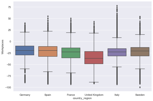
Let’s first summarise one mobility category — for example, workplaces mobility — for the six selected countries using a box plot. In seaborn, we use the function catplot which displays the relationship between a numerical and one or more categorical variables using several visual representations, including bar plot, box plot, and violin plot.
The catplot function has many parameters. You can access them by typing sns.catplot? in a code cell. These are the parameters we will need for our first plot:
x— Categorical variable, in our case the variable “country_region” containing the labels of the six countriesy— Numerical variable, in our case the variable “workplaces_percent_change_from_baseline”data—pandasDataFramekind— The kind of plot to draw. Options are: “strip”, “swarm”, “box”, “violin”, “boxen”, “point”, “bar”, or “count”height— Height (in inches) of the plotaspect— Aspect * height gives the width (in inches) of the plot
# Box plot of workplaces mobility trends in selected countries

sns.catplot(
    x="country_region",
    y="Workplaces",
    kind="box",
    data=mobility_trends_countries,
    height=6,
    aspect=1.5,
);
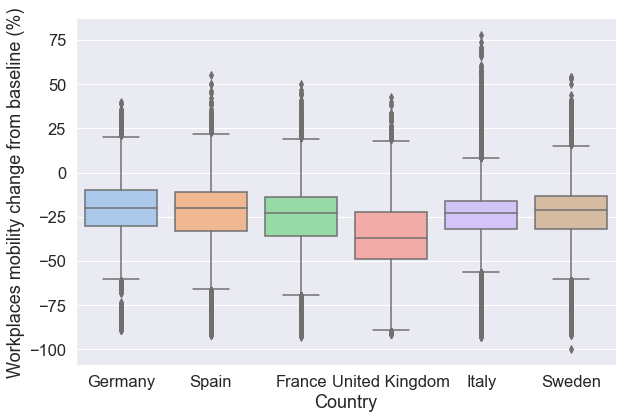
Changing figure appearance
Seaborn provides a range of capabilities to change figure appearance. For example, the figure below set a theme that controls color, font, and other features. The set_theme() function applies globally to the entire notebook so you do not need to execute again the function unless you want to change the theme. We also change the y and x axes labels.
# Control the scale of plot elements, font
sns.set_theme(context="notebook", style="darkgrid", palette="pastel", font_scale=1.5)

grid = sns.catplot(
    x="country_region",
    y="Workplaces",
    kind="box",
    data=mobility_trends_countries,
    height=6,
    aspect=1.5,
)

# Change the labels of the two axes
grid.set(xlabel="Country", ylabel="Workplaces mobility change from baseline (%)");
You can access information about the catplot function by typing help(sns.catplot) or sns.catplot?
sns.catplot?
Signature:
sns.catplot(
    *,
    x=None,
    y=None,
    hue=None,
    data=None,
    row=None,
    col=None,
    col_wrap=None,
    estimator=<function mean at 0x7fd028186a60>,
    ci=95,
    n_boot=1000,
    units=None,
    seed=None,
    order=None,
    hue_order=None,
    row_order=None,
    col_order=None,
    kind='strip',
    height=5,
    aspect=1,
    orient=None,
    color=None,
    palette=None,
    legend=True,
    legend_out=True,
    sharex=True,
    sharey=True,
    margin_titles=False,
    facet_kws=None,
    **kwargs,
)
Docstring:
Figure-level interface for drawing categorical plots onto a FacetGrid.

This function provides access to several axes-level functions that
show the relationship between a numerical and one or more categorical
variables using one of several visual representations. The ``kind``
parameter selects the underlying axes-level function to use:

Categorical scatterplots:

- :func:`stripplot` (with ``kind="strip"``; the default)
- :func:`swarmplot` (with ``kind="swarm"``)

Categorical distribution plots:

- :func:`boxplot` (with ``kind="box"``)
- :func:`violinplot` (with ``kind="violin"``)
- :func:`boxenplot` (with ``kind="boxen"``)

Categorical estimate plots:

- :func:`pointplot` (with ``kind="point"``)
- :func:`barplot` (with ``kind="bar"``)
- :func:`countplot` (with ``kind="count"``)

Extra keyword arguments are passed to the underlying function, so you
should refer to the documentation for each to see kind-specific options.

Note that unlike when using the axes-level functions directly, data must be
passed in a long-form DataFrame with variables specified by passing strings
to ``x``, ``y``, ``hue``, etc.

As in the case with the underlying plot functions, if variables have a
``categorical`` data type, the levels of the categorical variables, and
their order will be inferred from the objects. Otherwise you may have to
use alter the dataframe sorting or use the function parameters (``orient``,
``order``, ``hue_order``, etc.) to set up the plot correctly.

This function always treats one of the variables as categorical and
draws data at ordinal positions (0, 1, ... n) on the relevant axis, even
when the data has a numeric or date type.

See the :ref:`tutorial <categorical_tutorial>` for more information.

After plotting, the :class:`FacetGrid` with the plot is returned and can
be used directly to tweak supporting plot details or add other layers.

Parameters
----------
x, y, hue : names of variables in ``data``
    Inputs for plotting long-form data. See examples for interpretation.
data : DataFrame
    Long-form (tidy) dataset for plotting. Each column should correspond
    to a variable, and each row should correspond to an observation.
row, col : names of variables in ``data``, optional
    Categorical variables that will determine the faceting of the grid.
col_wrap : int
    "Wrap" the column variable at this width, so that the column facets
    span multiple rows. Incompatible with a ``row`` facet.
estimator : callable that maps vector -> scalar, optional
    Statistical function to estimate within each categorical bin.
ci : float or "sd" or None, optional
    Size of confidence intervals to draw around estimated values.  If
    "sd", skip bootstrapping and draw the standard deviation of the
    observations. If ``None``, no bootstrapping will be performed, and
    error bars will not be drawn.
n_boot : int, optional
    Number of bootstrap iterations to use when computing confidence
    intervals.
units : name of variable in ``data`` or vector data, optional
    Identifier of sampling units, which will be used to perform a
    multilevel bootstrap and account for repeated measures design.
seed : int, numpy.random.Generator, or numpy.random.RandomState, optional
    Seed or random number generator for reproducible bootstrapping.
order, hue_order : lists of strings, optional
    Order to plot the categorical levels in, otherwise the levels are
    inferred from the data objects.
row_order, col_order : lists of strings, optional
    Order to organize the rows and/or columns of the grid in, otherwise the
    orders are inferred from the data objects.
kind : str, optional
    The kind of plot to draw, corresponds to the name of a categorical
    axes-level plotting function. Options are: "strip", "swarm", "box", "violin",
    "boxen", "point", "bar", or "count".
height : scalar
    Height (in inches) of each facet. See also: ``aspect``.
aspect : scalar
    Aspect ratio of each facet, so that ``aspect * height`` gives the width
    of each facet in inches.
orient : "v" | "h", optional
    Orientation of the plot (vertical or horizontal). This is usually
    inferred based on the type of the input variables, but it can be used
    to resolve ambiguity when both `x` and `y` are numeric or when
    plotting wide-form data.
color : matplotlib color, optional
    Color for all of the elements, or seed for a gradient palette.
palette : palette name, list, or dict
    Colors to use for the different levels of the ``hue`` variable. Should
    be something that can be interpreted by :func:`color_palette`, or a
    dictionary mapping hue levels to matplotlib colors.
legend : bool, optional
    If ``True`` and there is a ``hue`` variable, draw a legend on the plot.
legend_out : bool
    If ``True``, the figure size will be extended, and the legend will be
    drawn outside the plot on the center right.
share{x,y} : bool, 'col', or 'row' optional
    If true, the facets will share y axes across columns and/or x axes
    across rows.
margin_titles : bool
    If ``True``, the titles for the row variable are drawn to the right of
    the last column. This option is experimental and may not work in all
    cases.
facet_kws : dict, optional
    Dictionary of other keyword arguments to pass to :class:`FacetGrid`.
kwargs : key, value pairings
    Other keyword arguments are passed through to the underlying plotting
    function.

Returns
-------
g : :class:`FacetGrid`
    Returns the :class:`FacetGrid` object with the plot on it for further
    tweaking.

Examples
--------

Draw a single facet to use the :class:`FacetGrid` legend placement:

.. plot::
    :context: close-figs

    >>> import seaborn as sns
    >>> sns.set_theme(style="ticks")
    >>> exercise = sns.load_dataset("exercise")
    >>> g = sns.catplot(x="time", y="pulse", hue="kind", data=exercise)

Use a different plot kind to visualize the same data:

.. plot::
    :context: close-figs

    >>> g = sns.catplot(x="time", y="pulse", hue="kind",
    ...                data=exercise, kind="violin")

Facet along the columns to show a third categorical variable:

.. plot::
    :context: close-figs

    >>> g = sns.catplot(x="time", y="pulse", hue="kind",
    ...                 col="diet", data=exercise)

Use a different height and aspect ratio for the facets:

.. plot::
    :context: close-figs

    >>> g = sns.catplot(x="time", y="pulse", hue="kind",
    ...                 col="diet", data=exercise,
    ...                 height=5, aspect=.8)

Make many column facets and wrap them into the rows of the grid:

.. plot::
    :context: close-figs

    >>> titanic = sns.load_dataset("titanic")
    >>> g = sns.catplot(x="alive", col="deck", col_wrap=4,
    ...                 data=titanic[titanic.deck.notnull()],
    ...                 kind="count", height=2.5, aspect=.8)

Plot horizontally and pass other keyword arguments to the plot function:

.. plot::
    :context: close-figs

    >>> g = sns.catplot(x="age", y="embark_town",
    ...                 hue="sex", row="class",
    ...                 data=titanic[titanic.embark_town.notnull()],
    ...                 orient="h", height=2, aspect=3, palette="Set3",
    ...                 kind="violin", dodge=True, cut=0, bw=.2)

Use methods on the returned :class:`FacetGrid` to tweak the presentation:

.. plot::
    :context: close-figs

    >>> g = sns.catplot(x="who", y="survived", col="class",
    ...                 data=titanic, saturation=.5,
    ...                 kind="bar", ci=None, aspect=.6)
    >>> (g.set_axis_labels("", "Survival Rate")
    ...   .set_xticklabels(["Men", "Women", "Children"])
    ...   .set_titles("{col_name} {col_var}")
    ...   .set(ylim=(0, 1))
    ...   .despine(left=True))  #doctest: +ELLIPSIS
    <seaborn.axisgrid.FacetGrid object at 0x...>
File:      ~/.local/lib/python3.8/site-packages/seaborn/categorical.py
Type:      function
Wide and long data format
In the original data, each mobility category is a separate column, which is known as wide data format. Wide data format is easy to read but restricts us to plotting only one mobility category at a time (unless we employ a for loop). We can plot all mobility categories simultaneously in seaborn after we reshape our data from wide format to long format. Long data format will have one column for all six mobility categories and one column for the values of those categories.
Below is a Pandas schematic of wide (left) and long format data (right):

Reshaping our mobility categories from wide to long format using the pandas melt function. The function transforms a DataFrame into a format where one or more columns are identifier variables (id_vars), while other columns (value_vars) are turned into a long format, returning columns, ‘variable’ and ‘value’. In our example, id_vars arecountry_region and date, and value_vars are the six mobility categories. The melt function takes the following parameters:
DataFrame— your pandas DataFrameid_vars— a list of identifier variablesvalue_vars— a list of variables to turn into long format
The code below also removes NaN, standing for Not a Number, using the method dropna()
Tip
Instead of manually creating a list of all six column labels for the six mobility categories of interest, you can obtain the list by typing in
mobility_trends_countries.columns[9:15]
where the attribute columns returns the column labels of the DataFrame mobility_trends_countries and the indices in square brackets [9:15] specify the location of the mobility categories’ columns of interest. The command returns the labels in the following format:
Index(['retail_and_recreation_percent_change_from_baseline',
       'grocery_and_pharmacy_percent_change_from_baseline',
       'parks_percent_change_from_baseline',
       'transit_stations_percent_change_from_baseline',
       'workplaces_percent_change_from_baseline',
       'residential_percent_change_from_baseline'],
      dtype='object')
# From wide to long format using the function melt
mobility_trends_countries_long = pd.melt(
    mobility_trends_countries,
    id_vars=["country_region", "sub_region_1", "date"],
    # The columns 'date' and 'sub_region_1' are not needed for the box
    # plots below but we will need the two variables in subsequent tasks.
    value_vars=mobility_trends_countries.columns[9:15],
).dropna()

mobility_trends_countries_long
| country_region | sub_region_1 | date | variable | value | |
|---|---|---|---|---|---|
| 502 | Germany | Baden-Württemberg | 2020-02-15 | Retail_Recreation | 6.0 |
| 503 | Germany | Baden-Württemberg | 2020-02-16 | Retail_Recreation | 23.0 |
| 504 | Germany | Baden-Württemberg | 2020-02-17 | Retail_Recreation | 0.0 |
| 505 | Germany | Baden-Württemberg | 2020-02-18 | Retail_Recreation | 4.0 |
| 506 | Germany | Baden-Württemberg | 2020-02-19 | Retail_Recreation | 2.0 |
| ... | ... | ... | ... | ... | ... |
| 2916551 | Sweden | Västra Götaland County | 2021-06-24 | Residential | 2.0 |
| 2916552 | Sweden | Västra Götaland County | 2021-06-25 | Residential | 9.0 |
| 2916555 | Sweden | Västra Götaland County | 2021-06-28 | Residential | 5.0 |
| 2916556 | Sweden | Västra Götaland County | 2021-06-29 | Residential | 4.0 |
| 2916557 | Sweden | Västra Götaland County | 2021-06-30 | Residential | 4.0 |
2446789 rows × 5 columns
The resulting DataFrame mobility_trends_countries_long contains two new columns: variable containing the six mobility categories per country per date, and value containing the values of those categories (percent change from baseline).
Multi-plot visualisations
To plot the six mobility categories simultaneously in a multi-plot, we simply add the parameter col and provide as an argument our categorical variable labeled variable. Our six mobility categories will be plotted in a grid of six columns. Setting the col_wrap parameter to 2 will plot the six variables in two columns, spanning three rows. We change the kind of plot we would like to draw to boxen.
# Differences in multiple mobility trends across selected countries
g = sns.catplot(
    x="country_region",
    y="value",
    col="variable",
    col_wrap=2,
    kind="boxen",
    height=6,
    aspect=1.5,  # control plot size
    data=mobility_trends_countries_long,
)
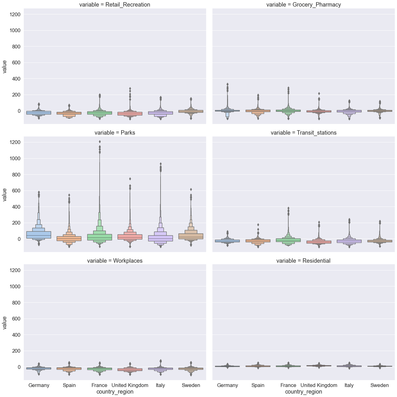
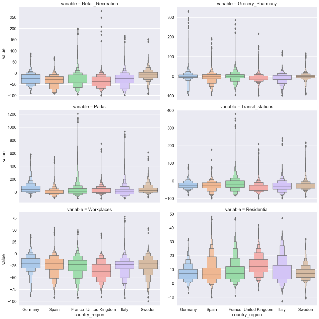
The plots above have one deficiency — different mobility categories share the same y axis. Because the axis range is predominantly determined by one mobility category (parks mobility) and its wide distribution, the plots barely display the way in which the six countries differ with respect to the remaining five mobility category. We resolve this problem by simply setting the parameter sharey to False and redrawing the figure.
sns.catplot(
    x="country_region",
    y="value",
    col="variable",
    col_wrap=2,
    kind="boxen",
    height=6,
    aspect=1.5,  # control plot size
    sharey=False,  # set different y axes for each plot
    data=mobility_trends_countries_long,
);
Hands-on exercise
Visualise mobility categories for a different set of countries of your choice. Update the labels and interpret your results. Employ a different kind of catplot, for example violin.
RQ2: How do mobility trends change over time?
Our graphics so far summarised the time series mobility data without visualising longitudinal trends. In this section, you will learn how to visualise time series data in order to characterise mobility trends across countries and along time.
Visualising time series data
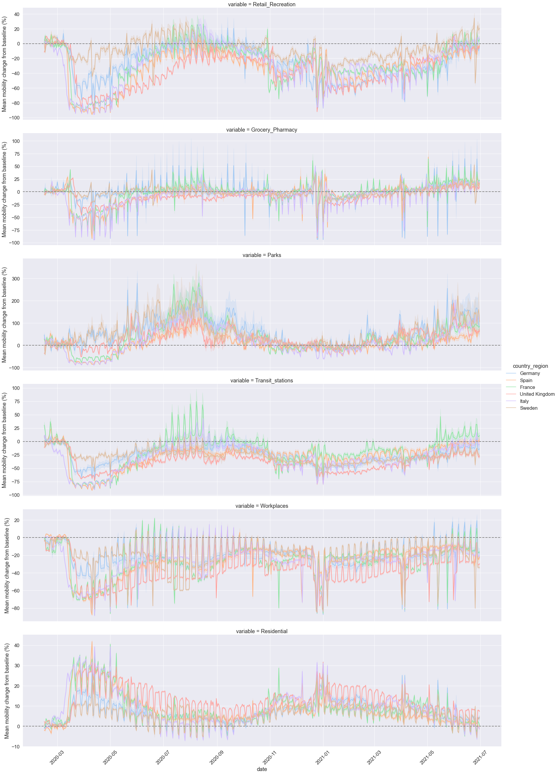
We will use the function relplot() for drawing relational plots onto a multi-plot grid. Using the function, we will produce six plots for the six mobility categories. Each plot will represent the relationship between two variables, time and mean mobility percent change from baseline.
Let’s have a look at the parameters:
x,y— Numerical variables on the x and y axes. We plotdateon the x axis and thevalueof percent mobility change from baseline on the y axis.hue— Grouping variable that will map elements to different colors. Our grouping variable iscountry_region, meaning that the line for each country will be colored differently.kind— Kind of plot to draw, with two options:scatter(default) andline. We uselinein order to visualise the trend in data.
The resulting plot shows the mean percent change and 99% confidence intervals for each mobility category. The 99% CI are computed using bootstrapping. Observations are sorted by time.
# Plot daily mobility trends across mobility categories and countries of interest

grid = sns.relplot(
    x="date",
    y="value",
    hue="country_region",
    col="variable",
    col_wrap=1,
    height=6,
    aspect=4,
    linewidth=2,
    ci=99,
    seed=42,
    facet_kws={"sharey": False, "sharex": True},
    kind="line",
    data=mobility_trends_countries_long,
)

grid.set(ylabel="Mean mobility change from baseline (%)")
grid.set_xticklabels(rotation=45)

# For each plot, draw a horizontal line at y = 0 representing the baseline
for ax in grid.axes.flat:
    ax.axhline(color="gray", linestyle="--", lw=2)
Bootstrapping for inference
We calculated above a point estimate — mean per cent mobility change from baseline — for each mobility category per day and per country between March 2020 and May 2021. The point estimate likely contains some error and thus, it rarely captures the exact population parameter. Therefore, in addition to our point estimate, we need to compute a range of plausible values that, with some degree of certainty, contains the true population parameter. This range of plausible values is called a confidence interval. Confidence intervals are typically constructed using confidence levels of 95% or 99%.
We compute the 99% confidence intervals around the mean, representing the uncertainty of the mean estimate. The 99% confidence interval is a range of plausible values that you can be 99% certain contain the true mean of the population parameter.
To construct confidence intervals on the mean (and other sample statistics), Seaborn uses a procedure called bootstrapping. The bootstrapping is a resampling method of statistical inference that is alternative to the classical approach of hypothesis testing. (Other resampling methods include random permutation.) The bootstrap method uses the original sample of our data to generate another random sample that resembles the population, following these steps:
Treat the original sample as if it were the population.
Draw from the sample, at random with replacement, the same number of times as the original sample size.

Source: Ani Adhikari and John DeNero (with David Wagner and Henry Milner). Computational and Inferential Thinking: The Foundations of Data Science.
In our example, the data for each mobility category and day within a country is treated as a sample on which bootstrapping on the mean is performed. After each bootstrap resample, the mean is computed, generating a distribution from where the confidence intervals for the mean are constructed.
When you compute bootstrap confidence intervals in Seaborn, you can set the following parameters:
ci— Confidence level that will determine the size of the confidence interval. Commonly used confidence levels include 95% and 99%. The default confidence level in the current version ofseabornis 95%.n-boot— Number of bootstrap resamples. By default,Seabornuses 1000 bootstrap resamples for computing the confidence intervals. You could set a greater number of bootstrap resamples — for example 10,000, by typingn_boot=10000— but keep in mind that increasing the number of resamples can be time-consuming for large data sets.seed— Seed reproducible bootstrapping. The easiest way is to specify an integer.
There are many good introductions to resampling methods (including bootstrapping) and inference. See the section on the Bootstrap in Ani Adhikari and John DeNero (with David Wagner and Henry Milner). Computational and Inferential Thinking: The Foundations of Data Science. Another useful resource is David Diez, Christopher Barr, Mine Cetinkaya-Rundel. Introductory Statistics with Randomization and Simulation, OpenIntro. See also the informative and entertaining talk by John Rauser Statistics Without the Agonizing Pain, Strata + Hadoop 2014, on using resampling methods for making inference.
RQ3: How have mobility trends differed across UK lockdowns?
Our next research question aims to explore differences in mobility trends across the three national lockdowns in the United Kingdom. Because the three lockdowns brought different measures, restrictions, and regulations, differences in mobility trends should not be interpreted as a direct indication of compliance or non-compliance with lockdown rules.
We will use the first three weeks of each lockdown to compare the three lockdowns. Let’s select the data for the first lockdown (24 March 2020 — 13 April 2020), second lockdown (5 November 2020 — 25 November 2020), and third lockdown (6 January 2021 — 26 January 2021) in the United Kingdom.
# Create three new DataFrames, each containing a subset of data about
# the first three weeks of the respective lockdown

first_lockdown_UK = mobility_trends_countries_long[
    (mobility_trends_countries_long["country_region"] == "United Kingdom")
    & (mobility_trends_countries_long["date"] >= "2020-03-24")
    & (mobility_trends_countries_long["date"] <= "2020-04-13")
]

second_lockdown_UK = mobility_trends_countries_long[
    (mobility_trends_countries_long["country_region"] == "United Kingdom")
    & (mobility_trends_countries_long["date"] >= "2020-11-05")
    & (mobility_trends_countries_long["date"] <= "2020-11-25")
]

third_lockdown_UK = mobility_trends_countries_long[
    (mobility_trends_countries_long["country_region"] == "United Kingdom")
    & (mobility_trends_countries_long["date"] >= "2021-01-06")
    & (mobility_trends_countries_long["date"] <= "2021-01-26")
]
# Show data about the first national lockdown in the UK
# (The dataframes for the other two lockdowns have the same number of columns)
first_lockdown_UK
| country_region | sub_region_1 | date | variable | value | |
|---|---|---|---|---|---|
| 95896 | United Kingdom | Aberdeen City | 2020-03-24 | Retail_Recreation | -75.0 |
| 95897 | United Kingdom | Aberdeen City | 2020-03-25 | Retail_Recreation | -78.0 |
| 95898 | United Kingdom | Aberdeen City | 2020-03-26 | Retail_Recreation | -80.0 |
| 95899 | United Kingdom | Aberdeen City | 2020-03-27 | Retail_Recreation | -80.0 |
| 95900 | United Kingdom | Aberdeen City | 2020-03-28 | Retail_Recreation | -87.0 |
| ... | ... | ... | ... | ... | ... |
| 2734968 | United Kingdom | York | 2020-04-06 | Residential | 28.0 |
| 2734969 | United Kingdom | York | 2020-04-07 | Residential | 28.0 |
| 2734970 | United Kingdom | York | 2020-04-08 | Residential | 28.0 |
| 2734971 | United Kingdom | York | 2020-04-09 | Residential | 28.0 |
| 2734972 | United Kingdom | York | 2020-04-10 | Residential | 33.0 |
48902 rows × 5 columns
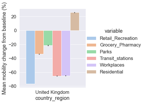
Visualising lockdowns’ mobility as barplots
Plot mean mobility change for the six mobility categories during the first lockdown in the UK using the Seaborn function catplot(). Error bars represent 95% confidence intervals.
grid = sns.catplot(
    kind="bar", x="country_region", y="value", hue="variable", data=first_lockdown_UK
)
grid.set(ylabel="Mean mobility change from baseline (%)")
# grid.set(ylim=(-80, 40)); uncomment to set the y axis to a particular range of values
<seaborn.axisgrid.FacetGrid at 0x7fd08feaee50>
Ideally, we would like to plot the three lockdowns as a multi-plot. To achieve this, we first concatenate the three DataFrames into one DataFrame using the Pandas concat() function. In addition, to add an identifier for each of three DataFrames in the new DataFrame, we specify their labels as a list for the parameter keys. We use the Pandas method reset_index() to add the three identifiers of the original lockdown DataFrames as a column ‘level_0’ in the new DataFrame.
lockdowns_dataframes = [first_lockdown_UK, second_lockdown_UK, third_lockdown_UK]
three_lockdowns_UK = pd.concat(
    lockdowns_dataframes,
    keys=["first_lockdown_UK", "second_lockdown_UK", "third_lockdown_UK"],
).reset_index()
three_lockdowns_UK
| level_0 | level_1 | country_region | sub_region_1 | date | variable | value | |
|---|---|---|---|---|---|---|---|
| 0 | first_lockdown_UK | 95896 | United Kingdom | Aberdeen City | 2020-03-24 | Retail_Recreation | -75.0 |
| 1 | first_lockdown_UK | 95897 | United Kingdom | Aberdeen City | 2020-03-25 | Retail_Recreation | -78.0 |
| 2 | first_lockdown_UK | 95898 | United Kingdom | Aberdeen City | 2020-03-26 | Retail_Recreation | -80.0 |
| 3 | first_lockdown_UK | 95899 | United Kingdom | Aberdeen City | 2020-03-27 | Retail_Recreation | -80.0 |
| 4 | first_lockdown_UK | 95900 | United Kingdom | Aberdeen City | 2020-03-28 | Retail_Recreation | -87.0 |
| ... | ... | ... | ... | ... | ... | ... | ... |
| 150176 | third_lockdown_UK | 2735259 | United Kingdom | York | 2021-01-22 | Residential | 23.0 |
| 150177 | third_lockdown_UK | 2735260 | United Kingdom | York | 2021-01-23 | Residential | 16.0 |
| 150178 | third_lockdown_UK | 2735261 | United Kingdom | York | 2021-01-24 | Residential | 14.0 |
| 150179 | third_lockdown_UK | 2735262 | United Kingdom | York | 2021-01-25 | Residential | 21.0 |
| 150180 | third_lockdown_UK | 2735263 | United Kingdom | York | 2021-01-26 | Residential | 22.0 |
150181 rows × 7 columns
We now visualise as a multi-plot grid the mean mobility trends and 95% CI for the three lockdowns in the United Kingdom. We specify the new categorical variable level_0 to determine the faceting of the multi-plot grid.
# Display the three lockdowns as a catplot multi-plot
grid = sns.catplot(
    kind="bar",
    x="country_region",
    y="value",
    hue="variable",
    col="level_0",
    data=three_lockdowns_UK,
)
grid.set_ylabels("Mean mobility change from baseline (%)")
<seaborn.axisgrid.FacetGrid at 0x7fcf8a34d820>
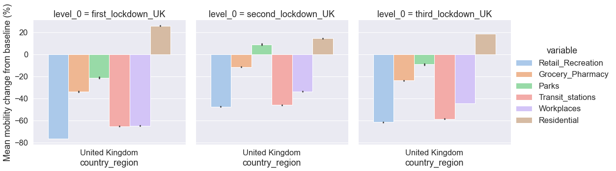
As a general tendency, the plots indicate that, on average, changes of mobility (compared to the baseline period in early 2020) during the first lockdown were greater that changes of mobility during the third lockdown, and both were greater than changes of mobility during the second lockdown.
Discussion activity
Different rules and restrictions were in place during the three lockdowns. Let’s discuss how those differences in restrictions were associated with differences in mobility during the three lockdowns across mobility categories.
RQ4: How have mobility trends differed across UK counties during the third lockdown?
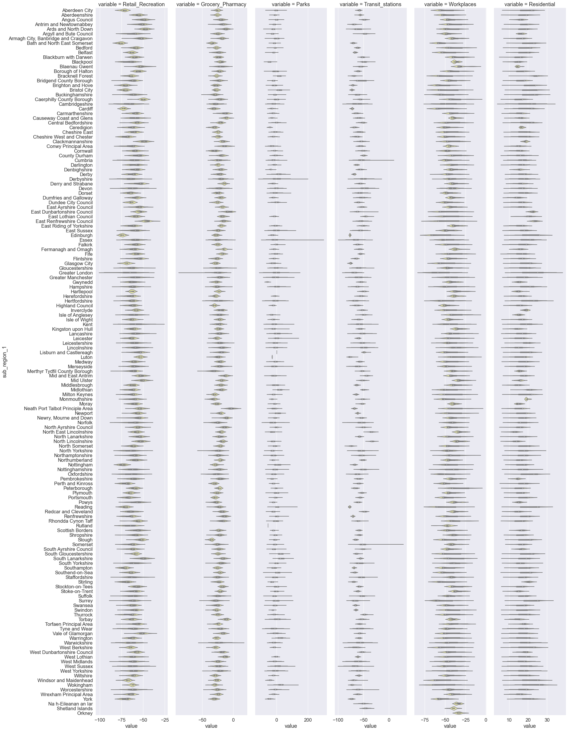
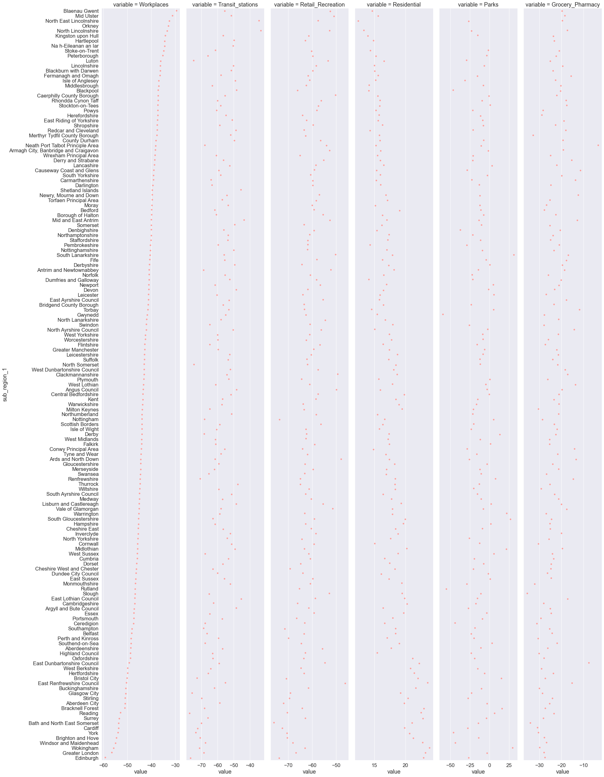
We will now explore mobility trends across mobility categories and counties in the United Kingdom during the third lockdown. We employ the Seaborn catplot() function using one of our DataFrame ‘third_lockdown_UK’. We use the variable called variable, which contains the labels of the six mobility categories to determine the faceting of the multi-plot grid. The UK counties are on the vertical axis and the mean values of mobility change from baseline (%) are on the horizontal axis. The violin plot function computes, for each pair of country and mobility category, the mean mobility change and the distributions of the mobility percent change.
Multi-plot visualisations
Note the simplicity of the code that produces the multi-plot and the richness of information it provides.
sns.catplot(
    x="value",
    y="sub_region_1",
    col="variable",
    kind="violin",
    sharex=False,
    height=35,
    aspect=0.13,
    color="y",
    data=third_lockdown_UK,
);
The above plots are slightly difficult to interpret because the values of mean mobility are not sorted. An elegant approach to sorting would be to employ Pandas functionality and then pass the sorted mean mobility values to a Seaborn plot.
Split-apply-combine
To calculate the mean mobility change per both UK county and mobility category, we first need to split the data into groups where each mobility category per county is a group. Then, second, we will apply a function to calculate the mean for each of the split groups (mobility category per county) such that the daily values over the lockdown period for each mobility category per county will be summarised into a single mean value. Third, we will combine the individual calculations for each split group into a single DataFrame. The procedure is known as split-apply-combine. We will use the Pandas method groupby() to perform the procedure on the mobility trends data.
Summarising data by groups
We first specify the variables to be used to determine the groups. In our example, these are ‘variable’ and ‘sub_region_1’, resulting in 876 groups (6 mobility categories times 146 UK counties). Because we want to split the data into groups by two variables, we pass the variables within the groupby() methods as a list ‘[‘variable’, ‘sub_region_1’]’. We then specify the variable on which we want to perform the calculation (in our case, take the mean) and compute the mean for each of the 876 groups using the mean() method. We use the Pandas method reset_index() at the end of the command in order to convert the output (from Series) to a DataFrame. The output DataFrame ‘third_lockdown_UK_mean’ contains three columns: mobility categories (‘variable’), counties (‘sub_region_1’), and the mean (‘value’). Each row is a pair of mobility category and county, and their respective mean mobility change calculated over the three weeks’ period.
# Compute grouped means using the Pandas gropupby() method
third_lockdown_UK_mean = (
    third_lockdown_UK.groupby(["variable", "sub_region_1"])["value"]
    .mean()
    .reset_index()
)
third_lockdown_UK_mean
| variable | sub_region_1 | value | |
|---|---|---|---|
| 0 | Grocery_Pharmacy | Aberdeen City | -25.333333 |
| 1 | Grocery_Pharmacy | Aberdeenshire | -26.190476 |
| 2 | Grocery_Pharmacy | Angus Council | -19.714286 |
| 3 | Grocery_Pharmacy | Antrim and Newtownabbey | -18.523810 |
| 4 | Grocery_Pharmacy | Ards and North Down | -13.285714 |
| ... | ... | ... | ... |
| 871 | Workplaces | Windsor and Maidenhead | -54.952381 |
| 872 | Workplaces | Wokingham | -55.714286 |
| 873 | Workplaces | Worcestershire | -42.469388 |
| 874 | Workplaces | Wrexham Principal Area | -38.428571 |
| 875 | Workplaces | York | -53.904762 |
876 rows × 3 columns
Our next step is to sort in decreasing order the UK counties within each mobility category by their values of mean mobility change. We use the Pandas method sort_values() to accomplish that:
third_lockdown_UK_mean_sorted = third_lockdown_UK_mean.sort_values(
    by=[
        "variable",
        "value",
    ],
    ascending=False,
)[["sub_region_1", "variable", "value"]]
third_lockdown_UK_mean_sorted
| sub_region_1 | variable | value | |
|---|---|---|---|
| 737 | Blaenau Gwent | Workplaces | -29.523810 |
| 803 | Mid Ulster | Workplaces | -31.142857 |
| 816 | North East Lincolnshire | Workplaces | -32.523810 |
| 825 | Orkney | Workplaces | -32.866667 |
| 818 | North Lincolnshire | Workplaces | -33.380952 |
| ... | ... | ... | ... |
| 25 | Ceredigion | Grocery_Pharmacy | -31.142857 |
| 83 | Monmouthshire | Grocery_Pharmacy | -32.095238 |
| 77 | Merthyr Tydfil County Borough | Grocery_Pharmacy | -32.761905 |
| 7 | Bath and North East Somerset | Grocery_Pharmacy | -34.095238 |
| 112 | Slough | Grocery_Pharmacy | -35.523810 |
876 rows × 3 columns
We now plot the mean mobility change across UK counties sorted by Workplaces mobility in decreasing order. We can easily see, for example, that workplaces mobility was the most reduced in Edinburgh and Greater London. However, counties were sorted only in the Workplaces mobility category while in the remaining categories counties follow the ranking as specified in Workplaces mobility.
g = sns.catplot(
    x="value",
    y="sub_region_1",
    col="variable",
    kind="strip",
    sharex=False,
    height=35,
    aspect=0.13,
    color="r",
    data=third_lockdown_UK_mean_sorted,
)
Typically, we are interested in computing multiple descriptive statistics in addition to the mean (e.g., median). We can compute multiple descriptive statistics using the Pandas method agg(). The code below is similar to the one we used to compute the mean on groups but this time we do not compute only the mean but many descriptive statistics at once. Specifically, we create a list of all the descriptive statistics we are interested in computing [min, max, np.mean, np.median, np.std] which is then passed inside the brackets of the agg() method. Note that some descriptive statistics are computed using built-in functions from the Python Standard Library (e.g., min and max) while others are computed using NumPy functions (e.g., np.mean, np.median, and np.std). The resulting DataFrame contains a column for each descriptive statistic in addition to the grouping columns ‘sub_region_1’ and ‘variable’.
third_lockdown_UK_descriptive_stats = (
    third_lockdown_UK.groupby(["sub_region_1", "variable"])["value"]
    .agg([min, max, np.mean, np.median, np.std])
    .reset_index()
)
third_lockdown_UK_descriptive_stats
| sub_region_1 | variable | min | max | mean | median | std | |
|---|---|---|---|---|---|---|---|
| 0 | Aberdeen City | Grocery_Pharmacy | -33.0 | -20.0 | -25.333333 | -24.0 | 2.921187 |
| 1 | Aberdeen City | Parks | -51.0 | 42.0 | -3.142857 | -4.0 | 20.060622 |
| 2 | Aberdeen City | Residential | 11.0 | 24.0 | 19.809524 | 22.0 | 4.319943 |
| 3 | Aberdeen City | Retail_Recreation | -79.0 | -68.0 | -72.047619 | -71.0 | 3.138092 |
| 4 | Aberdeen City | Transit_stations | -64.0 | -55.0 | -58.619048 | -58.0 | 2.290768 |
| ... | ... | ... | ... | ... | ... | ... | ... |
| 871 | York | Parks | -63.0 | -22.0 | -46.190476 | -45.0 | 10.975514 |
| 872 | York | Residential | 13.0 | 25.0 | 20.666667 | 22.0 | 3.799123 |
| 873 | York | Retail_Recreation | -78.0 | -64.0 | -70.571429 | -69.0 | 4.307800 |
| 874 | York | Transit_stations | -78.0 | -69.0 | -73.380952 | -74.0 | 2.578298 |
| 875 | York | Workplaces | -60.0 | -41.0 | -53.904762 | -57.0 | 6.847662 |
876 rows × 7 columns
Let’s put in use the descriptive statistics indices we created. For example, we can determine the UK county with the most reduced median Retail and Recreation mobility during the third lockdown. We first access all the rows about Retail and Recreation mobility. We then use the Pandas sort_values function to sort all counties by their median mobility change in decreasing order. The output shows that Bath and North East Somerset is the county with the most reduced Retail and Recreation mobility during the third lockdown.
third_lockdown_UK_descriptive_stats[
    third_lockdown_UK_descriptive_stats["variable"] == "Retail_Recreation"
].sort_values(by="median")
| sub_region_1 | variable | min | max | mean | median | std | |
|---|---|---|---|---|---|---|---|
| 44 | Bath and North East Somerset | Retail_Recreation | -82.0 | -71.0 | -76.000000 | -76.0 | 2.898275 |
| 575 | Nottingham | Retail_Recreation | -80.0 | -68.0 | -73.619048 | -74.0 | 3.513918 |
| 284 | Edinburgh | Retail_Recreation | -78.0 | -69.0 | -73.809524 | -74.0 | 2.400397 |
| 126 | Cardiff | Retail_Recreation | -77.0 | -67.0 | -72.523810 | -73.0 | 2.441701 |
| 3 | Aberdeen City | Retail_Recreation | -79.0 | -68.0 | -72.047619 | -71.0 | 3.138092 |
| ... | ... | ... | ... | ... | ... | ... | ... |
| 114 | Caerphilly County Borough | Retail_Recreation | -64.0 | -46.0 | -50.238095 | -50.0 | 3.871754 |
| 167 | Clackmannanshire | Retail_Recreation | -57.0 | -42.0 | -49.352941 | -49.0 | 4.076475 |
| 15 | Angus Council | Retail_Recreation | -58.0 | -41.0 | -49.904762 | -49.0 | 4.380694 |
| 27 | Ards and North Down | Retail_Recreation | -56.0 | -41.0 | -47.857143 | -47.0 | 3.650832 |
| 266 | East Renfrewshire Council | Retail_Recreation | -55.0 | -35.0 | -46.190476 | -47.0 | 4.331501 |
148 rows × 7 columns
We can use the above commands to find any value of interest. For example, we can find the county with the greatest increase of Parks mobility from baseline by using the max value and accessing data about the Parks mobility category.
third_lockdown_UK_descriptive_stats[
    third_lockdown_UK_descriptive_stats["variable"] == "Parks"
].sort_values(by="max", ascending=False)
| sub_region_1 | variable | min | max | mean | median | std | |
|---|---|---|---|---|---|---|---|
| 288 | Essex | Parks | -69.0 | 270.0 | -3.511737 | -12.0 | 45.749895 |
| 213 | Derbyshire | Parks | -86.0 | 168.0 | 0.476744 | -4.5 | 45.763114 |
| 330 | Greater London | Parks | -94.0 | 131.0 | -3.167376 | -3.0 | 35.234568 |
| 412 | Leicester | Parks | -24.0 | 110.0 | 5.666667 | 1.0 | 28.812035 |
| 628 | Reading | Parks | -29.0 | 101.0 | 6.526316 | 1.0 | 28.083939 |
| ... | ... | ... | ... | ... | ... | ... | ... |
| 847 | Windsor and Maidenhead | Parks | -63.0 | -27.0 | -43.666667 | -42.0 | 9.640194 |
| 436 | Luton | Parks | -30.0 | -29.0 | -29.333333 | -29.0 | 0.577350 |
| 148 | Ceredigion | Parks | -56.0 | -33.0 | -43.857143 | -43.0 | 6.966245 |
| 342 | Gwynedd | Parks | -71.0 | -45.0 | -59.714286 | -61.0 | 6.827466 |
| 651 | Rutland | Parks | -55.0 | -55.0 | -55.000000 | -55.0 | 0.000000 |
135 rows × 7 columns
RQ5: How do mobility categories relate to each other?
We will now visualise distributions of the six mobility categories and examine similarities and differences as well as relationships between the distributions of mobility categories. We can use a histogram to visualise the distribution of mobility categories. The code below employs the Seaborn histplot() function to plot the distribution of Workplaces mobility in the UK since mid-February 2020 as a histogram.
# We first select data for the UK only
mobility_trends_UK = mobility_trends[
    mobility_trends["country_region"] == "United Kingdom"
]
mobility_trends_UK.head()
| country_region_code | country_region | sub_region_1 | sub_region_2 | metro_area | iso_3166_2_code | census_fips_code | place_id | date | Retail_Recreation | Grocery_Pharmacy | Parks | Transit_stations | Workplaces | Residential | |
|---|---|---|---|---|---|---|---|---|---|---|---|---|---|---|---|
| 3577753 | GB | United Kingdom | NaN | NaN | NaN | NaN | NaN | ChIJqZHHQhE7WgIReiWIMkOg-MQ | 2020-02-15 | -12.0 | -7.0 | -35.0 | -12.0 | -4.0 | 2.0 |
| 3577754 | GB | United Kingdom | NaN | NaN | NaN | NaN | NaN | ChIJqZHHQhE7WgIReiWIMkOg-MQ | 2020-02-16 | -7.0 | -6.0 | -28.0 | -7.0 | -3.0 | 1.0 |
| 3577755 | GB | United Kingdom | NaN | NaN | NaN | NaN | NaN | ChIJqZHHQhE7WgIReiWIMkOg-MQ | 2020-02-17 | 10.0 | 1.0 | 24.0 | -2.0 | -14.0 | 2.0 |
| 3577756 | GB | United Kingdom | NaN | NaN | NaN | NaN | NaN | ChIJqZHHQhE7WgIReiWIMkOg-MQ | 2020-02-18 | 7.0 | -1.0 | 20.0 | -3.0 | -14.0 | 2.0 |
| 3577757 | GB | United Kingdom | NaN | NaN | NaN | NaN | NaN | ChIJqZHHQhE7WgIReiWIMkOg-MQ | 2020-02-19 | 6.0 | -2.0 | 8.0 | -4.0 | -14.0 | 3.0 |
Visualising distributions
# Plot the distribution of the Workplaces mobility category as a histogram
ax = sns.histplot(mobility_trends_UK["Workplaces"], bins=10)

# Change the label of the horizontal axis
ax.set(xlabel="Mean workplaces mobility in the UK");
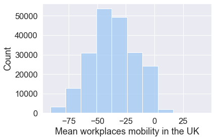
The distribution of Workplaces mobility appears symmetric, meaning that the left side of the distribution largely mirrors the right side.
In addition, we can use the histplot() to compare any two or more distributions by plotting them simultaneously.
# Plot two (or more) variables as histograms in a single plot
plt.figure(figsize=(16, 12))
sns.histplot(
    mobility_trends_UK[["Workplaces", "Retail_Recreation"]], alpha=0.4, bins=20
)
<AxesSubplot:ylabel='Count'>
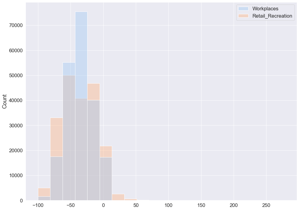
Both distributions appear symmetric. The distribution of Retail and Recreation mobility is slightly wider compared to the distribution of Workplaces mobility which is more centered around the mean. We can examine the distributions further by computing the mean and the standard deviation of mobility change in the UK across the six mobility categories since mid-February 2020.
Mean mobility change in the UK across mobility categories.
mobility_trends_UK.iloc[:, 9:15].mean()
Retail_Recreation   -36.809680
Grocery_Pharmacy     -8.658667
Parks                28.105415
Transit_stations    -38.142992
Workplaces          -35.856338
Residential          12.764187
dtype: float64
Standard deviation (std) of mobility change in the UK across mobility categories.
mobility_trends_UK.iloc[:, 9:15].std()
Retail_Recreation    26.273590
Grocery_Pharmacy     16.426443
Parks                54.650707
Transit_stations     23.548502
Workplaces           19.692586
Residential           7.421347
dtype: float64
These outputs confirm that the distribution of Retail and Recreation mobility is slightly wider (std = 25.1) compared to the distribution of Workplaces mobility (std = 19.7).
Plotting pairwise relationships
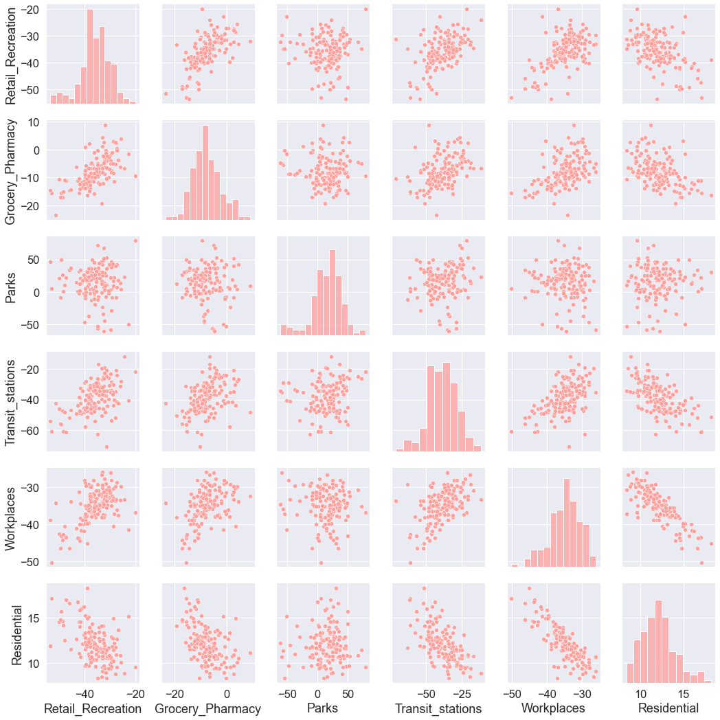
You can obtain a summary of interesting pairwise relationships between mobility categories in your data set. In Seaborn, PairGrid allows you to draw a grid of small subplots where each row and column corresponds to a different variable. The resulting grid displays all the pairwise relationships in the data set. In the case of mobility data, the plot displays all pairwise relationships between the mean mobility change for each mobility category in the United Kingdom since mid February 2020. Each data point in the plots below represents a UK county. The plot enables a quick examination of pairwise relationships between those mean mobility changes across counties, and makes easy to determine in an ‘open-minded’ manner apparent positive relationships, negative relationships, or no relationships.
# Compute the mean mobility change for each mobility category across UK counties
mobility_trends_UK_mean = mobility_trends_UK.groupby("sub_region_1")[
    [
        "Retail_Recreation",
        "Grocery_Pharmacy",
        "Parks",
        "Transit_stations",
        "Workplaces",
        "Residential",
    ]
].mean()

# Check the data in the DataFrame of mean mobility change we computed
mobility_trends_UK_mean.head()
| Retail_Recreation | Grocery_Pharmacy | Parks | Transit_stations | Workplaces | Residential | |
|---|---|---|---|---|---|---|
| sub_region_1 | ||||||
| Aberdeen City | -50.046371 | -10.722567 | 20.557692 | -46.127016 | -42.489919 | 14.567010 |
| Aberdeenshire | -28.253669 | -11.248447 | 22.474684 | -39.953878 | -37.207661 | 12.222222 |
| Angus Council | -25.955975 | -6.125786 | 13.982143 | -31.150943 | -33.542339 | 10.831551 |
| Antrim and Newtownabbey | -29.377358 | -7.465409 | -29.134328 | -53.752621 | -33.679435 | 12.859031 |
| Ards and North Down | -27.262055 | 0.452830 | 6.838298 | -41.721311 | -35.991935 | 12.679039 |
# Draw a multi-grid scatterplots of pairwise relationships
grid = sns.PairGrid(mobility_trends_UK_mean)
grid.map(sns.scatterplot, color="r")
<seaborn.axisgrid.PairGrid at 0x7fd04f09d6a0>
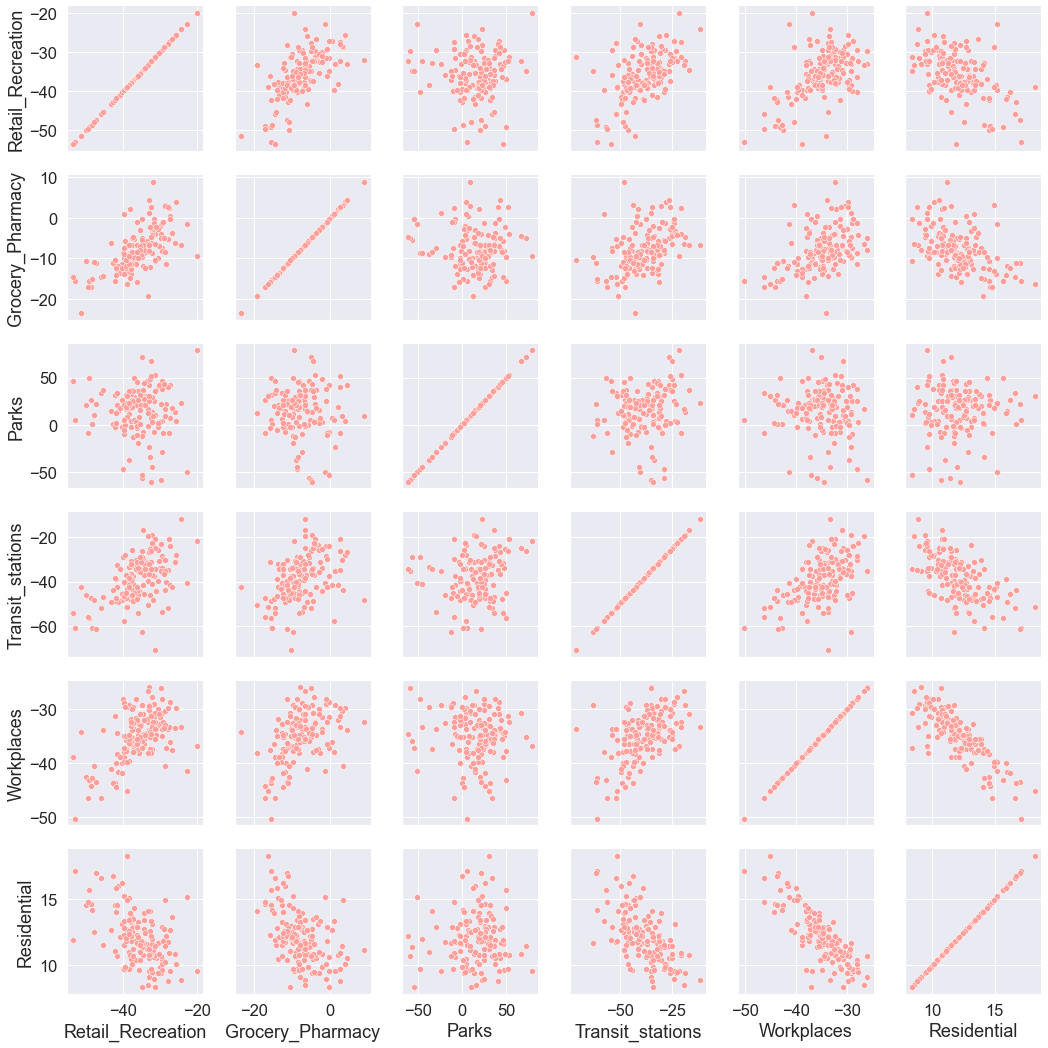
The information on the diagonal is not informative as it shows how a variable is correlated with itself. Instead, we could display a histogram on the diagonal representing the distribution of each mobility category.
# Draw a multi-plot of scatterplots representing pairwise relationships
grid = sns.PairGrid(mobility_trends_UK_mean)
grid.map_diag(sns.histplot, color="r")
grid.map_offdiag(sns.scatterplot, color="r")
<seaborn.axisgrid.PairGrid at 0x7fcf928a1940>
Interpreting pairwise relationships
Let’s interpret the pairwise relationships between the mean mobility trends. Which mobility trends appear to be involved in:
positive relationship
negative relationship
no relationship
Recall that each data point represents a UK county.
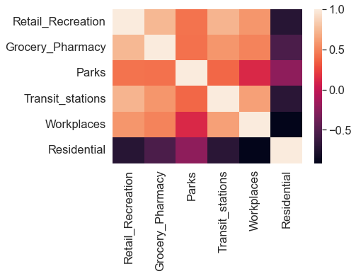
Visualising correlation
# Plot a heatmap based on the correlation analysis
sns.heatmap(mobility_trends_UK_corr);
We now fit a toy linear regression model using the linregress() function from the SciPy.stats module. We regress residential mobility on workplaces mobility.
# Fit a linear regression model and store results
slope, intercept, r_value, p_value, std_err = stats.linregress(
    x=mobility_trends_UK["Workplaces"], y=mobility_trends_UK["Residential"]
)
slope, intercept, r_value, p_value, std_err
(nan, nan, nan, nan, nan)
The linregress() failed to return model output. This is because the function does not deal well with Not a Number (NaN) values. A straightforward solution during the exploratory phase of analysis is to remove NaNs. However, other approaches may be more informative at the modelling stage, including mean imputation. We perform mean imputation by replacing missing values of a variable by the mean computed on the non-missing observations of that variable.
# Number of rows and columns in the DataFrame with NaNs
mobility_trends_UK.shape
(209033, 15)
mobility_trends_UK_NADrop = mobility_trends_UK.dropna(
    subset=[
        "country_region",
        "sub_region_1",
        "date",
        "Retail_Recreation",
        "Grocery_Pharmacy",
        "Parks",
        "Transit_stations",
        "Workplaces",
        "Residential",
    ]
)

# Number of rows and columns in the DataFrame without NaNs
mobility_trends_UK_NADrop.shape
(150757, 15)
The dropna() function removes one quarter of the rows. In subsequent analysis, it would make sense to impute missing values, including a simple procedure for replacing NaNs with the mean value for that county and mobility category.
Below we fit again a linear regression model using the new DataFrame that contain no NaN values.
# Fit a linear regression model and display outputs
model_outputs = stats.linregress(
    mobility_trends_UK_NADrop["Workplaces"], mobility_trends_UK_NADrop["Residential"]
)
model_outputs
LinregressResult(slope=-0.35580786753641186, intercept=0.3745693881369405, rvalue=-0.9297780751627193, pvalue=0.0, stderr=0.00036281934265285695)
model_outputs.slope
-0.35580786753641186
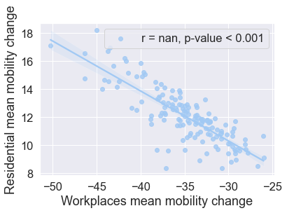
Visualising linear regression
We now plot a regression line and 95% confidence interval using the Seaborn regplot function. We also include in a legend the correlation coefficient and the actual p-value. The p-value from the linear regression model outputs reads 0. The p-value, however, is never a 0. P-values less than .001 are typically reported as as P<.001, instead of the actual exact p-value. We indicate this in the visualisation below.
# Visualise a linear relationship between Workplaces mobility and Residential mobility

fig = sns.regplot(
    x="Workplaces",
    y="Residential",
    label="r = {0:.3}, p-value < {1:.3}".format(r_value, 0.001),
    data=mobility_trends_UK_mean,
)
fig.set(
    xlabel="Workplaces mean mobility change", ylabel="Residential mean mobility change"
)
fig.legend()
<matplotlib.legend.Legend at 0x7fcf92818520>
We used above the SciPy module to fit a linear least-squares regression model. There is another library in Python, Statsmodels, which is widely used for statistical analysis.
For completeness, we fit the same linear least-squares regression model as above using the Statsmodels function OLS. Recall that we gave the Statsmodels library the alias sm when we imported the library at the top of the notebook.
# Rerun the ordinary least squares (OLS) regression  using the Statsmodels library

X = sm.add_constant(mobility_trends_UK_NADrop["Workplaces"])
Y = mobility_trends_UK_NADrop["Residential"]
model = sm.OLS(Y, X)
results = model.fit()
results

results.summary()
print_model = results.summary()
print(print_model)
                            OLS Regression Results
==============================================================================
Dep. Variable:            Residential   R-squared:                       0.864
Model:                            OLS   Adj. R-squared:                  0.864
Method:                 Least Squares   F-statistic:                 9.617e+05
Date:                Wed, 04 May 2022   Prob (F-statistic):               0.00
Time:                        09:47:58   Log-Likelihood:            -3.7043e+05
No. Observations:              150757   AIC:                         7.409e+05
Df Residuals:                  150755   BIC:                         7.409e+05
Df Model:                           1
Covariance Type:            nonrobust
==============================================================================
                 coef    std err          t      P>|t|      [0.025      0.975]
------------------------------------------------------------------------------
const          0.3746      0.015     25.247      0.000       0.345       0.404
Workplaces    -0.3558      0.000   -980.675      0.000      -0.357      -0.355
==============================================================================
Omnibus:                     4300.991   Durbin-Watson:                   0.595
Prob(Omnibus):                  0.000   Jarque-Bera (JB):             5567.433
Skew:                          -0.340   Prob(JB):                         0.00
Kurtosis:                       3.651   Cond. No.                         83.4
==============================================================================

Notes:
[1] Standard Errors assume that the covariance matrix of the errors is correctly specified.
Recording dependencies
# Install the watermark extension
!pip install -q watermark

# Load the watermark extension
%load_ext watermark

# Show packages that were imported
%watermark --iversions
matplotlib : 3.3.2
statsmodels: 0.12.2
scipy      : 1.5.2
seaborn    : 0.11.2
pandas     : 1.1.3
numpy      : 1.19.2
Save a list of the packages (and their versions) used in the current notebook to a file named requirements.txt.
!pipreqsnb ../notebooks/05_data_exploration_and_visualisation.ipynb
Exception occurred while working on file ../notebooks/05_data_exploration_and_visualisation.ipynb, cell 23/98
Traceback (most recent call last):
  File "/Users/valentindanchev/opt/anaconda3/bin/pipreqsnb", line 8, in <module>
    sys.exit(main())
  File "/Users/valentindanchev/opt/anaconda3/lib/python3.8/site-packages/pipreqsnb/pipreqsnb.py", line 129, in main
    raise e
  File "/Users/valentindanchev/opt/anaconda3/lib/python3.8/site-packages/pipreqsnb/pipreqsnb.py", line 126, in main
    imports += get_import_string_from_source(source)
  File "/Users/valentindanchev/opt/anaconda3/lib/python3.8/site-packages/pipreqsnb/pipreqsnb.py", line 26, in get_import_string_from_source
    tree = ast.parse(source)
  File "/Users/valentindanchev/opt/anaconda3/lib/python3.8/ast.py", line 47, in parse
    return compile(source, filename, mode, flags,
  File "<unknown>", line 1
    sns.catplot?
               ^
SyntaxError: invalid syntax