.ipynb .pdf

repository open issue

Binder

Contents

Network analysis with NetworkX

This lab provides an introduction to the study of social networks. Network data and network analysis focus on the relationships between entities, including individuals, organisations, countries, and other entities. In the course so far, the data we have studied were from different sources, including digital, administrative, and survey sources, but with one common feature — these were tabular data. Tabular data is structured into rows, each representing a distinct observation (e.g., individuals, counties) and columns representing observations’ attributes. By contrast, in network data we are not primarily interested in the attributes of distinct observations but in the relationships between those observations.

A network is a set of nodes (also called vertices) and a set of edges (also called links) between them. In networks, nodes represent individuals (or other entities, including countries, organisations, and Web pages) and links represent various social ties, including friendship, kinship, acquaintanceship, or hyperlinks.

Network analysis studies the patterns of relationships that emerge from the interaction of individuals or other entities. Such patterns are often described as network structure. Network structure can be characterised at different scales:

• local scale (e.g., nodes, dyads, and triads)

• meso-scale (e.g., network communities)

• macro-scale (e.g., network diameter)

Different metrics and methods have been developed to measure properties of network structure at the local, meso, and macro scales. For example, community detection methods have been developed to study meso-scale network structure.

The rationale of network analysis is that the position of a node in a network affects relevant social outcomes, for example node importance and performance in a social system. An overview of network analysis can be found in Wasserman and Faust (1994) and Newman (2018).

In this lab, we will first create and study a small toy network in order to build an intuition about basic network concepts and diagnostics. We will then study a social network of characters in the movie Star Wars Episode IV: A New Hope.

Learning resources

Stephen Borgatti, Ajay Mehra, Daniel Brass, Giuseppe Labianca. 2009. Network Analysis in the Social Sciences. Science.

Petter Holme, Mason A. Porter, Hiroki Sayama. Who Is the Most Important Character in Frozen? What Networks Can Tell Us About the World. Frontiers for Young Minds.

Mark Newman. 1. The Connected World and 2. What Networks Can Tell Us About the World. Santa Fe Institute.

Rob Chew’s and Peter Baumgartner Connected: A Social Network Analysis Tutorial with NetworkX. PyData 2016. Authors’ Jupyter notebooks are available on GitHub.

Menczer, F., Fortunato, S., Davis, C. 2020. A First Course in Network Science. Cambridge University Press. Authors’ Jupyter notebooks are available on GitHub.

Edward L. Platt. 2020. Network Science with Python and NetworkX Quick Start Guide: Explore and visualize network data effectively. Packt Publishing. Author’s Jupyter notebooks are available on GitHub.

Santo Fortunato and Darko Hric. 2016. Community detection in networks: A user guide.. Physics Reports. An open access version of the article is available on the arXiv.

Mason A. Porter, Jukka-Pekka Onnela, Peter J. Mucha. 2009. Communities in Networks. Notices of the AMS.

Valentin Danchev and Mason A. Porter. 2018. Neither global nor local: Heterogeneous connectivity in spatial network structures of world migration. Social Networks.

NetworkX tutorial.

Networks and COVID-19

Mapping the Social Network of Coronavirus. New York Times.

David Holtz et al. Interdependence and the cost of uncoordinated responses to COVID-19. PNAS.

S. Chang, E. Pierson, P. W. Koh, J. Gerardin, B. Redbird, D. Grusky, J. Leskovec. Mobility network models of COVID-19 explain inequities and inform reopening. Nature.

Open network data repositories

• Network Repository. An Interactive Scientific Network Data Repository.

• Mark Newman’s website

• Pajek datasets

• Stanford Large Network Dataset Collection

• Moviegalaxies—Social networks in movies

NetworkX

We will perform network analysis using NetworkX. NetworkX is a Python library for creating, analysing, and visualising networks:

• written in pure Python

• flexible and easy to install

• relatively scalable

Other Python libraries for network analysis

• python-igraph

  • written in C/C++ with interfaces to Python and R

  • pros: performance and speed; cons: installation can be a hurdle

• graph-tool

  • written in C++

  • fast algorithms and powerful visualisations

• Pymnet: Multilayer Networks Library for Python

  • written in Python, based on Matplotlib and integrated with NetworkX

  • handle multilayer networks: analysis and visualisation

Network representations

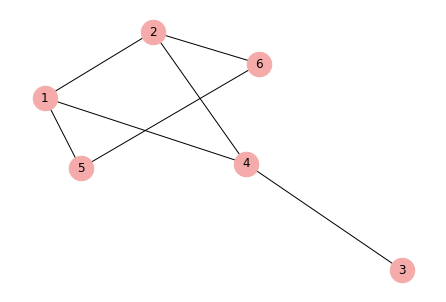
Below are four different representations of a network. Those four different network representations refer to the same set of nodes and the same set of edges connecting those nodes.

In the network, each person is a node. For example, Nancy is a node (ID 3) connected to three other nodes: Emma (ID 2), John (ID 4), and Emily (ID 5). Those three people are neighbors of Nancy. In network terms, Nancy has a degree of three. Similarly, Sophie has two neighbors (i.e., nodes to which Sophie is connected) so we say she has a degree of two.

This is an example of a simple network. Simple networks are characterised as:

• Undirected — edges between each pair of nodes have no direction such that if an edge from node A to node B is present, the edge from B to A is also present. By contrast, in directed networks, edges point to only one direction.

• Unweighted — edges between each pair of nodes are either present or absent. By contrast, in weighted networks, edges have weights assigned to them.

# Import Networkx and other packages we will use

import matplotlib.pyplot as plt
import networkx as nx
import pandas as pd
from scipy.stats.stats import pearsonr

%matplotlib inline

Creating an undirected network

We begin by creating an empty undirected network using Graph() in networkx (We already imported networkx as nx). The created empty network has no nodes and no edges.

# Create an empty network
G = nx.Graph()
# G = nx.DiGraph()  # To create a directed network

Let’s add a colection of nodes.

# Add nodes
G.add_node(1)

# Alternatively, you can add a set of nodes from a list
G.add_nodes_from([2, 3, 4, 5, 6])

Let’s now add a collection of edges connecting the nodes.

# Add edges
G.add_edge(1, 2)
G.add_edge(1, 4)

# Alternatively, you can add a set of edges from a list
G.add_edges_from([(1, 5), (2, 4), (2, 6), (3, 4), (5, 6)])

# Check the created edges
G.edges()

EdgeView([(1, 2), (1, 4), (1, 5), (2, 4), (2, 6), (3, 4), (5, 6)])

Examine basic properties of the graph using the info() function.

# Check basic properties of the graph
print(nx.info(G))

Graph with 6 nodes and 7 edges

<ipython-input-6-30b69dc9c89c>:2: DeprecationWarning: info is deprecated and will be removed in version 3.0.

  print(nx.info(G))

# Draw a network
nx.draw(G, with_labels=True, node_color="#F4ABAA", node_size=600)
plt.savefig("GraphUndirected.png", dpi=600)

Computing network diagnostics

We compute various network diagnostics, ranging from local (node-level) diagnostics (degree centrality) to global (network-level) diagnostics (e.g., network diameter).

Node-level diagnostics

Node degree

Node degree is simply the number of connections a node has.

# Compute node degree
nx.degree(G)

DegreeView({1: 3, 2: 3, 3: 1, 4: 3, 5: 2, 6: 2})

# Print node degree in a more readable format
for node in G.nodes:
    print(node, nx.degree(G, node))

1 3
2 3
3 1
4 3
5 2
6 2

Number of triangles

Number of triangles refers to any three connected nodes that include a node.

# Compute the number of triangles per node
for node in G.nodes:
    print(node, nx.triangles(G, node))

1 1
2 1
3 0
4 1
5 0
6 0

Clustering

Clustering of a node is the fraction of possible triangles (i.e., the number of actual triangles divided by the number of possible triangles).

# Compute the clustering coefficient for nodes
for node in G.nodes:
    print(node, nx.clustering(G, node))

1 0.3333333333333333
2 0.3333333333333333
3 0
4 0.3333333333333333
5 0
6 0

Let’s consolidate our code and print the above local network diagnostics in one place

# Multiple network diagnostics
print("node degree triangles clustering")
for node in nx.nodes(G):
    print(node, nx.degree(G, node), nx.triangles(G, node), nx.clustering(G, node))

node degree triangles clustering
1 3 1 0.3333333333333333
2 3 1 0.3333333333333333
3 1 0 0
4 3 1 0.3333333333333333
5 2 0 0
6 2 0 0

The above node-level diagnostics consider only direct connections to a node without taking into account the global structure of a network. Let’s compute diagnostics that take into account the global structure of our network.

Betweenness centrality and shortest paths

One such diagnostic is betweenness centrality. Nodes with high betweenness centrality are thought to connect otherwise disconnected nodes and in this sense to harness coordination and communication flow in social networks.

How do we compute betweenness centrality? Consider that between any pair of nodes there is a shortest path connected that pair, the betweenness centrality of a node is the sum of the fraction of shortest paths between all pairs that pass through a node.

To make things concrete, let’s first compute the shortest paths between a pair of nodes that go through a node. For example, the shortest paths that go through node 1: 2 → 5, 3 → 5, 4 → 5.

# Compute the shortest paths that go through a node
for i in range(2, 5):
    print(list(nx.all_shortest_paths(G, source=i, target=5)))

[[2, 1, 5], [2, 6, 5]]
[[3, 4, 1, 5]]
[[4, 1, 5]]

Let’s compute now the betweenness centrality for node 1.

The shortest paths, which pass through node 1, are between the pairs:

2 → 5

3 → 5

4 → 5

Pairs of nodes	Number of shortest paths through node 1	Number of all shortest paths
2 → 5	1	2
3 → 5	1	1
4 → 5	1	1

Betweenness centrality for node 1 is then computed as:

\(1/2 + 1/1 + 1/1 = 2.5\)

# Compute betweenness centrality
nx.betweenness_centrality(G, normalized=False)

{1: 2.5, 2: 2.5, 3: 0.0, 4: 4.0, 5: 0.5, 6: 0.5}

If normalized = True, then betweenness centrality of a node is normalised by \(((n - 1)(n - 2))/2\). In our example graph:

\(((6 - 1)(6 - 2))/2 = (5 * 4)/2 = 20 / 2 = 10\).

Hence the normalized betweenness centrality of, for example, node 1 is \(2.5/10 = 0.25\).

# Compute normalized betweenness centrality
nx.betweenness_centrality(G, normalized=True)

{1: 0.25, 2: 0.25, 3: 0.0, 4: 0.4, 5: 0.05, 6: 0.05}

Eigenvector centrality

Eigenvector centrality is another diagnostic that considers non-direct connections. If node degree measures the number of connections of a node, eigenvector centrality measures the extent to which those connected to a node are themselves highly connected nodes. Eigenvector centrality is an indicator of the influence of a node in a network. People with high eigenvector centrality in social and information networks are influential because they are connected to others who are themselves highly connected and, thus, can easily reach many other people in the networks.

# Compute eigenvector centrality
nx.eigenvector_centrality(G)

{1: 0.5131199170225811,
 2: 0.5131199170225811,
 3: 0.18452474299639904,
 4: 0.4726682070377605,
 5: 0.3285964750170798,
 6: 0.3285964750170798}

In our small undirected network, node 1 and node 2 have the highest eigenvector centrality due to their connections to each other and to node 4, each of which has degree of 3 and is therefore highly connected in this network of six nodes.

Network-level diagnostics

We now consider network-level diagnostics.

Average shortest path

One diagnostic that characterises the global structure of a network is the average shortest path for the network.

# Compute the average shortest path for the network
nx.average_shortest_path_length(G)

1.6666666666666667

Network diameter

Network diameter is another network-level diagnostic. Diameter of a network is the longest of all the path lengths or the maximum distance between nodes in a network.

nx.algorithms.distance_measures.diameter(G)

3

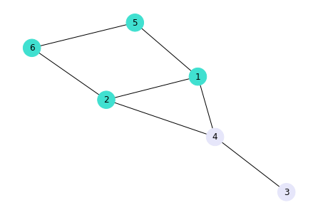
Assortative mixing

Assortativity or assortative mixing (also called homophily) is the preference of nodes with similar attributes to interact between each other. In other words, “similarity breeds connection” McPherson et al. Am. Soc. Rew.. To illustrate the tendency for assortative mixing, we first add node attributes.

Adding node attributes

# Add gender attribute to existing nodes
G.nodes[1]["gender"] = "female"
G.nodes[2]["gender"] = "female"
G.nodes[3]["gender"] = "male"
G.nodes[4]["gender"] = "male"
G.nodes[5]["gender"] = "female"
G.nodes[6]["gender"] = "female"

# Assign different colour to nodes with different attribute classes
nodes_colors = []
for node in G.nodes:
    if G.nodes[node]["gender"] == "female":
        nodes_colors.append("#40E0D0")
    else:
        nodes_colors.append("#E6E6FA")

# The resulting list of colors for female ('#a5b41f') and male ('#1fb4a5')
nodes_colors

['#40E0D0', '#40E0D0', '#E6E6FA', '#E6E6FA', '#40E0D0', '#40E0D0']

Plot the network with node colours representing gender categories

nx.draw(G, with_labels=True, node_color=nodes_colors, node_size=600)

# Save the graph
plt.savefig("GraphUndirectedGender.png", dpi=600)

Measuring assortativity

Let’s see if indeed similarity with respect to gender attributes breeds connections in our toy network. Networks in which similar nodes are more likely to connect than dissimilar nodes are called assortative.

# Compute assortativity coefficient
nx.attribute_assortativity_coefficient(G, attribute="gender")

0.29999999999999977

Nodes may be linked because they have similar social attributes but also because they have similar number of links or a similar role in a network. Let’s see if nodes with similar node degree are more likely (i.e., degree assortativity) or less likely (i.e., degree disassortativity) to be linked in our example network.

# Assortativity for node degree
nx.degree_assortativity_coefficient(G)

-0.10526315789473463

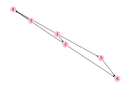
Creating a directed network

# Create an empty directed network
DG = nx.DiGraph()

# Add nodes
DG.add_nodes_from([1, 2, 3, 4, 5, 6])

# Add edges
DG.add_edges_from([(1, 2), (1, 4), (1, 5), (2, 4), (2, 6), (3, 4), (5, 6)])

# Draw the directed network
nx.draw(DG, with_labels=True, node_color="#FFC0CB", node_size=400)

# Save the graph
plt.savefig("GraphDirected.png", dpi=600)

# Compute out-degree and in-degree
print("node out_degree out_degree")
for node in nx.nodes(DG):
    print(node, DG.out_degree(node), DG.in_degree(node))

node out_degree out_degree
1 3 0
2 2 1
3 1 0
4 0 3
5 1 1
6 0 2

# Compute betweenness_centrality
nx.betweenness_centrality(DG, normalized=True)

{1: 0.0, 2: 0.025, 3: 0.0, 4: 0.0, 5: 0.025, 6: 0.0}

Discussion: How network diagnostics differ across directed and undirected networks?

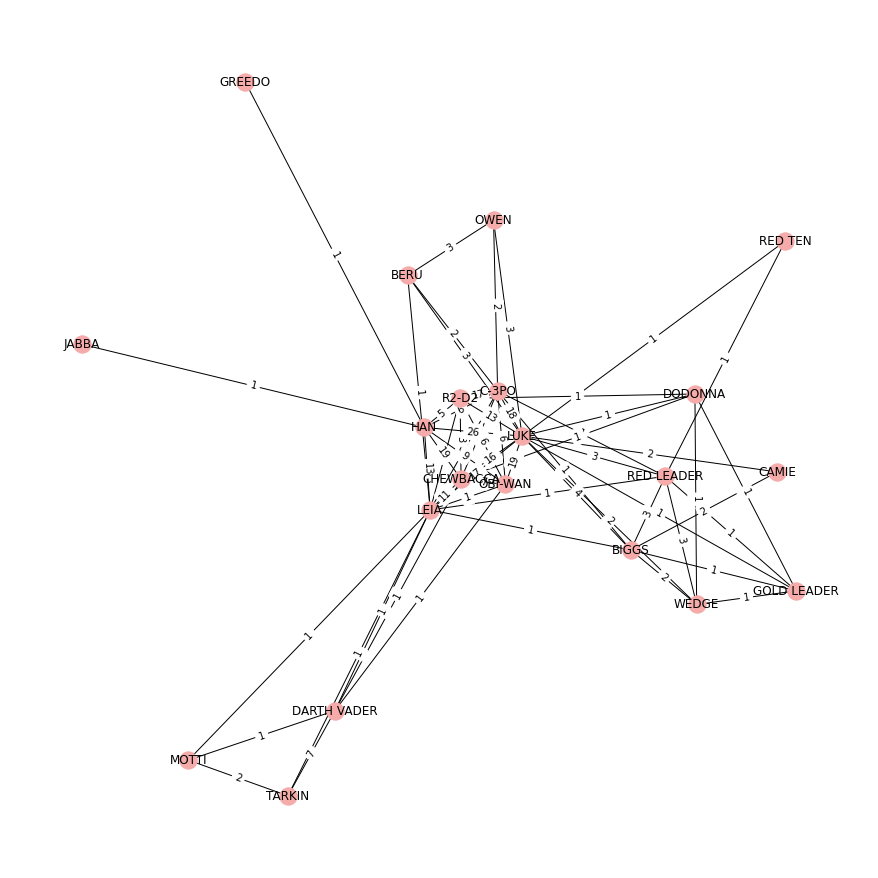
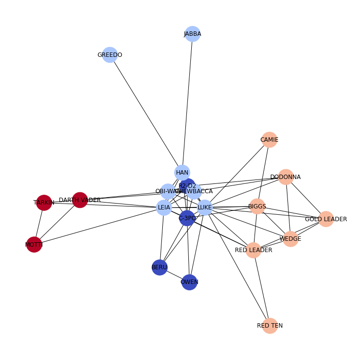
A fun example—Star Wars network

In this section we use a small weighted network reconstructed from the movie Star Wars Episode IV: A New Hope by Evelina Gabasova. The network is also used in the network analysis’ tutorial in R by Alex Hanna, Pablo Barbera, and Dan Cervone. For interactive social networks of characters in films and series, see the website Moviegalaxies.com.

Each node in the Star Wars Episode IV: A New Hope network represents a character and each edge represents the number of times a pair of characters appeared together in a scene of the movie. Edges are undirected and weighted.

We use a version of the edge list file named star-wars-network.csv (the file can also be found on this GitHub repository by Pablo Barberá), which we read using the Pandas function read_csv().

StarWars_df = pd.read_csv(
    "https://raw.githubusercontent.com/valdanchev/reproducible-data-science-python/master/data/star-wars-network.csv"
)
StarWars_df.head()

	source	target	weight
0	C-3PO	R2-D2	17
1	LUKE	R2-D2	13
2	OBI-WAN	R2-D2	6
3	LEIA	R2-D2	5
4	HAN	R2-D2	5

We now create a graph object using the NetworkX function from_pandas_edgelist()

GraphStarWars = nx.from_pandas_edgelist(
    StarWars_df, source="source", target="target", edge_attr=True
)

# Check the graph
print(nx.info(GraphStarWars))

Graph with 21 nodes and 60 edges

<ipython-input-31-24cf5aa5bfee>:2: DeprecationWarning: info is deprecated and will be removed in version 3.0.

  print(nx.info(GraphStarWars))

# Returns the number of edges in a network
GraphStarWars.size()

60

# Returns total weight sum
GraphStarWars.size(weight="weight")

295.0

# Check the weight of the edge between a pair of nodes
GraphStarWars["C-3PO"]["R2-D2"]["weight"]

17

# Specify figure size
plt.figure(figsize=(12, 12))

# Compute node position using the default spring_layout
node_position = nx.spring_layout(GraphStarWars)

# Draw the Star Wars Episode IV network
nx.draw(GraphStarWars, node_position, node_color="#F4ABAA", with_labels=True)

# Add edge weights
edge_labels = nx.get_edge_attributes(GraphStarWars, "weight")
nx.draw_networkx_edge_labels(GraphStarWars, node_position, edge_labels=edge_labels)

# Save the graph
plt.savefig("GraphStarWars.png", dpi=600)

Global network diagnostics

Let’s compute the average shortest path to characterise the global structure of the network. Recall that the average shortest path determines the extent to which characters in the Star Wars network are distant from one another.

# Compute the average shortest path for the network
nx.average_shortest_path_length(GraphStarWars)

1.9095238095238096

The other global diagnostic we consider is network diameter. Recall that the diameter of a network is the longest of all the path lengths or the maximum distance between nodes in a network.

nx.algorithms.distance_measures.diameter(GraphStarWars)

3

Meso-scale network diagnostics

To study the meso-scale properties of a network, we identify network communities. Network communities are collection of nodes that are more connected to each other than to other communities compared to a null model. Many community detection methods have been developed to identify community structure in networks. To identify network communities in the Star Wars network, we will use a technique called modularity maximisation. We will maximise modularity using the Louvain community detection heuristics.

# Install and import the Louvain community detection algorithm.
!pip install python-louvain
import community as community_louvain

# Detect the community structure of the graph which
# maximises the modularity using the Louvain heuristices.
partition = community_louvain.best_partition(GraphStarWars, resolution=1)

Requirement already satisfied: python-louvain in /Users/valentindanchev/opt/anaconda3/lib/python3.8/site-packages (0.14)
Requirement already satisfied: networkx in /Users/valentindanchev/.local/lib/python3.8/site-packages (from python-louvain) (2.8.5)
Requirement already satisfied: numpy in /Users/valentindanchev/opt/anaconda3/lib/python3.8/site-packages (from python-louvain) (1.19.2)

[notice] A new release of pip available: 22.2 -> 22.3.1
[notice] To update, run: pip install --upgrade pip

# Set figure size that is larger than the default
plt.figure(figsize=(10, 10))

nx.draw(
    GraphStarWars,
    with_labels=True,
    pos=nx.spring_layout(GraphStarWars),  # spring_layout is the default layout
    node_color=list(partition.values()),
    cmap=plt.cm.coolwarm,
    node_size=1000,
)

# Save the graph
plt.savefig("GraphStarWars.png", dpi=600)

Local network diagnostics

# Compute node degree (i.e., the number of edges adjacent to that node)
for node in GraphStarWars.nodes:
    print(node, nx.degree(GraphStarWars, node))

C-3PO 10
R2-D2 7
LUKE 15
OBI-WAN 7
LEIA 12
HAN 8
CHEWBACCA 8
DODONNA 5
DARTH VADER 5
CAMIE 2
BIGGS 7
BERU 4
OWEN 3
MOTTI 3
TARKIN 3
GREEDO 1
JABBA 1
GOLD LEADER 5
WEDGE 5
RED LEADER 7
RED TEN 2

# Sort the node degrees in descending order
GraphStarWars_degrees = nx.degree(GraphStarWars)
sorted(GraphStarWars_degrees, key=lambda x: x[1], reverse=True)

[('LUKE', 15),
 ('LEIA', 12),
 ('C-3PO', 10),
 ('HAN', 8),
 ('CHEWBACCA', 8),
 ('R2-D2', 7),
 ('OBI-WAN', 7),
 ('BIGGS', 7),
 ('RED LEADER', 7),
 ('DODONNA', 5),
 ('DARTH VADER', 5),
 ('GOLD LEADER', 5),
 ('WEDGE', 5),
 ('BERU', 4),
 ('OWEN', 3),
 ('MOTTI', 3),
 ('TARKIN', 3),
 ('CAMIE', 2),
 ('RED TEN', 2),
 ('GREEDO', 1),
 ('JABBA', 1)]

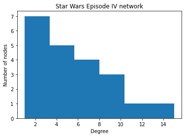
# Plot a histogram for node degrees
degree_values = dict(GraphStarWars_degrees).values()

plt.hist(degree_values, 6)
plt.xlabel("Degree")
plt.ylabel("Number of nodes")
plt.title("Star Wars Episode IV network")

Text(0.5, 1.0, 'Star Wars Episode IV network')

# Compute node strenght (i.e., the sum of the edge weights adjacent to a node)
gsw_weights = nx.degree(GraphStarWars, weight="weight")
sorted(gsw_weights, key=lambda x: x[1], reverse=True)

[('LUKE', 129),
 ('HAN', 80),
 ('C-3PO', 64),
 ('CHEWBACCA', 63),
 ('LEIA', 59),
 ('R2-D2', 50),
 ('OBI-WAN', 49),
 ('BIGGS', 14),
 ('RED LEADER', 13),
 ('DARTH VADER', 11),
 ('TARKIN', 10),
 ('BERU', 9),
 ('WEDGE', 9),
 ('OWEN', 8),
 ('DODONNA', 5),
 ('GOLD LEADER', 5),
 ('CAMIE', 4),
 ('MOTTI', 4),
 ('RED TEN', 2),
 ('GREEDO', 1),
 ('JABBA', 1)]

# Compute the number of triangles
triangles = nx.triangles(GraphStarWars)
sorted(triangles.items(), key=lambda x: x[1], reverse=True)[0:10]

[('LUKE', 35),
 ('LEIA', 27),
 ('C-3PO', 24),
 ('CHEWBACCA', 19),
 ('R2-D2', 17),
 ('OBI-WAN', 17),
 ('HAN', 15),
 ('BIGGS', 12),
 ('RED LEADER', 12),
 ('GOLD LEADER', 8)]

# Compute clustering
clustering = nx.clustering(GraphStarWars)
sorted(clustering.items(), key=lambda x: x[1], reverse=True)[0:10]

[('CAMIE', 1.0),
 ('OWEN', 1.0),
 ('MOTTI', 1.0),
 ('TARKIN', 1.0),
 ('RED TEN', 1.0),
 ('BERU', 0.8333333333333334),
 ('R2-D2', 0.8095238095238095),
 ('OBI-WAN', 0.8095238095238095),
 ('GOLD LEADER', 0.8),
 ('WEDGE', 0.8)]

# Compute the average shortest path for the network
nx.average_shortest_path_length(GraphStarWars)

1.9095238095238096

# Get the distance from one character (e.g., Luke) to any other character
nx.shortest_path_length(GraphStarWars, "LUKE")

{'LUKE': 0,
 'GOLD LEADER': 1,
 'CAMIE': 1,
 'R2-D2': 1,
 'C-3PO': 1,
 'BIGGS': 1,
 'DODONNA': 1,
 'CHEWBACCA': 1,
 'OWEN': 1,
 'WEDGE': 1,
 'OBI-WAN': 1,
 'BERU': 1,
 'LEIA': 1,
 'HAN': 1,
 'RED LEADER': 1,
 'RED TEN': 1,
 'GREEDO': 2,
 'JABBA': 2,
 'TARKIN': 2,
 'DARTH VADER': 2,
 'MOTTI': 2}

# Get the shortes path between any two characters
nx.shortest_path(GraphStarWars, "LUKE", "DARTH VADER")

['LUKE', 'CHEWBACCA', 'DARTH VADER']

# Compute betweenness centrality — unweighted
betweenness = nx.betweenness_centrality(GraphStarWars, normalized=False)
sorted(betweenness.items(), key=lambda x: x[1], reverse=True)[0:10]

[('LUKE', 62.428571428571416),
 ('LEIA', 45.59523809523809),
 ('HAN', 37.0),
 ('C-3PO', 12.095238095238093),
 ('CHEWBACCA', 7.452380952380952),
 ('BIGGS', 6.749999999999999),
 ('RED LEADER', 6.749999999999999),
 ('OBI-WAN', 3.119047619047619),
 ('R2-D2', 2.5),
 ('DARTH VADER', 2.5)]

# Compute betweenness centrality — weighted
betweenness = nx.betweenness_centrality(
    GraphStarWars, weight="weight", normalized=False
)
sorted(betweenness.items(), key=lambda x: x[1], reverse=True)[0:10]

[('LEIA', 59.95000000000001),
 ('DODONNA', 47.53333333333333),
 ('HAN', 37.0),
 ('C-3PO', 32.78333333333333),
 ('BIGGS', 31.91666666666667),
 ('RED LEADER', 31.416666666666668),
 ('GOLD LEADER', 23.799999999999997),
 ('R2-D2', 22.75),
 ('LUKE', 18.333333333333332),
 ('CHEWBACCA', 15.916666666666664)]

# Compute eigenvector centrality
eigenvector = nx.eigenvector_centrality(GraphStarWars)
sorted(eigenvector.items(), key=lambda x: x[1], reverse=True)[0:10]

[('LUKE', 0.41738499895449294),
 ('LEIA', 0.3621476171212343),
 ('C-3PO', 0.34237759659841116),
 ('CHEWBACCA', 0.2930928555695595),
 ('R2-D2', 0.2768558557532187),
 ('OBI-WAN', 0.2735423861677878),
 ('HAN', 0.2652851070021197),
 ('BIGGS', 0.2276935565670028),
 ('RED LEADER', 0.2276935565670028),
 ('DODONNA', 0.16949029608351718)]

References

• Menczer, F., Fortunato, S., Davis, C. 2020. A first course in network science. Cambridge University Press.

• Rob Chew’s and Peter Baumgartner’s tutorial Connected: A Social Network Analysis Tutorial with NetworkX. PyData 2016.

• Edward L. Platt. 2020. Network Science with Python and NetworkX Quick Start Guide: Explore and visualize network data effectively. Packt Publishing.

• Evelina Gabasova. 2015. The Star Wars social network.

Introduction to Causal Inference Data Ethics, Bias, and Fairness